Vectorizing multimodal e-commerce product data with AWS Titan: a practical guide


Learn how to transform e-commerce product data into numerical vectors using AWS Titan.
This guide show you how to use a multimodal model to create embeddings from both text and images, enabling better search, recommendations, and data analysis.
Introduction
This is a step-by-step practical guide on how to generate embeddings using AWS Titan multimodal model.
You'll learn how vectorization converts your product data into numerical representations, setting the stage for a chatbot or AI agent.
What you'll learn
By the end of this guide, you'll be able to:
- Use multimodal models to work with both text and images
- Convert product data into vectors with AWS Titan
- Build a basic vector search for better product recommendations
Prerequisites
This guide is designed for developers with some familiarity with Python. To follow along you'll need:
1. Python & Jupyter Notebook
- We'll write all code in a Jupyter Notebook environment
- You'll use a pre-prepared dataset with shoe product data and images
2. AWS Titan Multimodal Model
- We'll use AWS Titan to generate embeddings - a numerical representation for both text and images
Meet SoleMates: our example store
For this guide, we use SoleMates, a fictional online shoe store, to provide a real-world context for our examples.
All code and data relate to SoleMates, making it easier to follow along and apply the concepts:

SoleMates is our fictional online shoe store
Install dependencies
We use several libraries and packages in this guide.
Clone Github repository
I've prepared a Github repository with product data for our made-up shoe store SoleMates, start by cloning the Github repo.
The image folder with all the shoe images for SoleMates is 134.2 MB
Clone the GitHub repository to get started, run this command in your terminal:
git clone https://github.com/norahsakal/solemates-data.git
Then, navigate to the cloned repository folder:
cd solemates-data
Inside you'll find:
- CSV file:
data/solemates_shoe_directory.csv(product data) - For convenience, a pre-embedded dataset with all text and image embeddings is also available:
data/solemates_shoe_directory_with_embeddings_token_count.csv - Image folder: footwear (contains shoe images, ~134 MB)
Pip install Python dependencies
Next, pip install all the required Python packages:
pip install boto3 botocore ipython numpy pandas scikit-learn tqdm ipywidgets
After installation, go ahead and launch Jupyter Notebook and create a new empty Jupyter Notebook.
Run this in your terminal:
jupyter notebook

Launch Jupyter Notebook and create a new Notebook
Add Python imports
Before we start to work with our shoe data, add all the necessary Python imports in the first cell of your Jupyter Notebook:
import ast
import base64
from datetime import datetime
import json
import os

import boto3
from botocore.exceptions import NoCredentialsError

from IPython.display import display, Image, HTML

import numpy as np
import pandas as pd
from sklearn.metrics.pairwise import cosine_similarity
from tqdm import tqdm
from tqdm.autonotebook import tqdm
Load shoe data
First, load the SoleMates shoe dataset into a Pandas DataFrame.
We read the CSV file, convert the color_details column from a string to a list, and display the first few rows.
Go ahead and load the shoe dataset:
# Load the SoleMates shoe dataset
df_shoes = pd.read_csv('data/solemates_shoe_directory.csv')

# Convert 'color_details' from string representation of a list to an actual list
df_shoes['color_details'] = df_shoes['color_details'].apply(ast.literal_eval)

# Display the first few rows of the dataset
df_shoes.head()
You'll see this table in your Notebook:
| product_title | gender | product_type | color | usage | color_details | heel_height | heel_type | price_usd | brand | product_id | image |
|---|---|---|---|---|---|---|---|---|---|---|---|
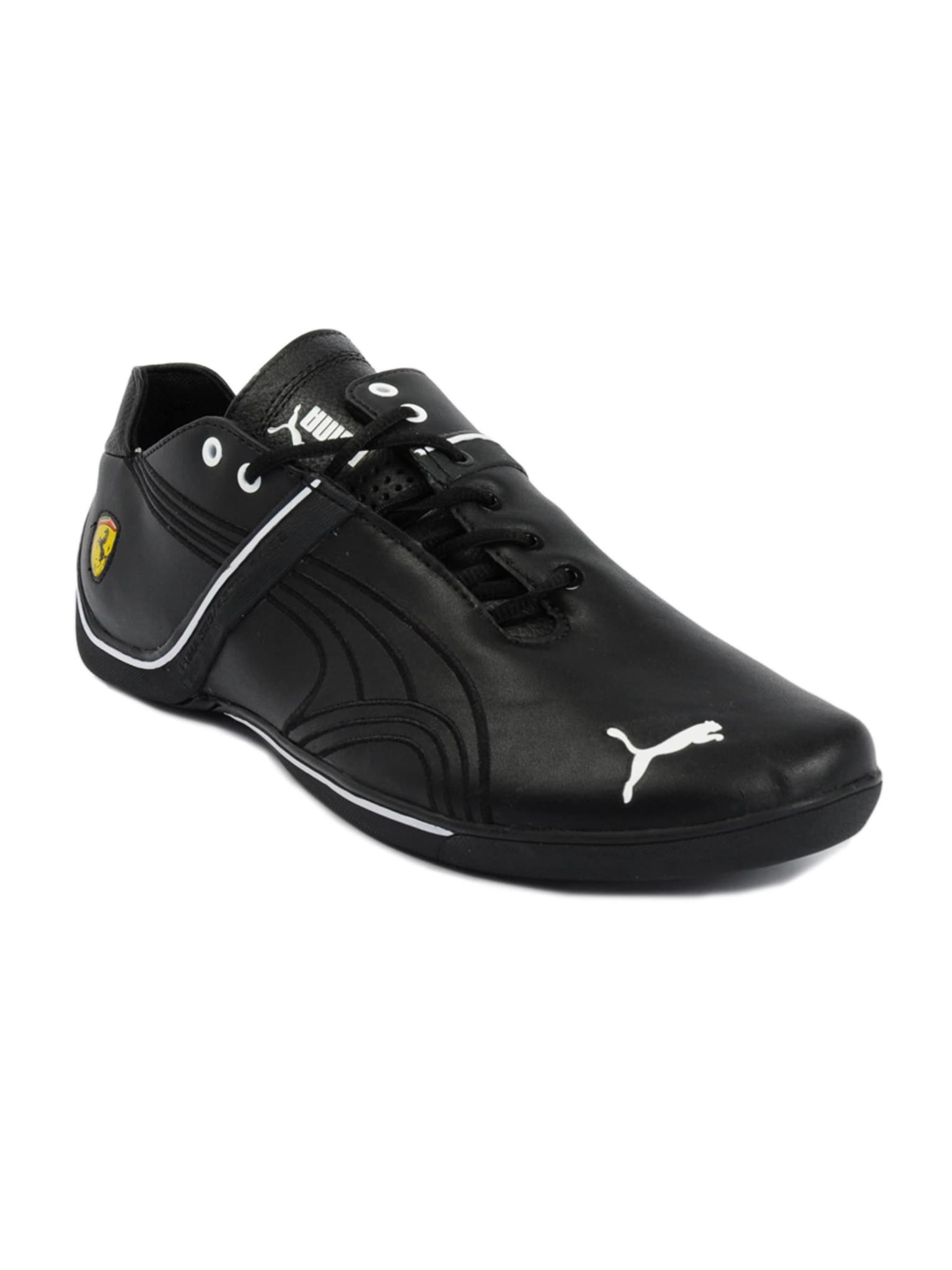
| Puma men future cat remix sf black casual shoes | men | casual shoes | black | casual | [] | nan | nan | 220 | puma | 1 | 1.jpg |
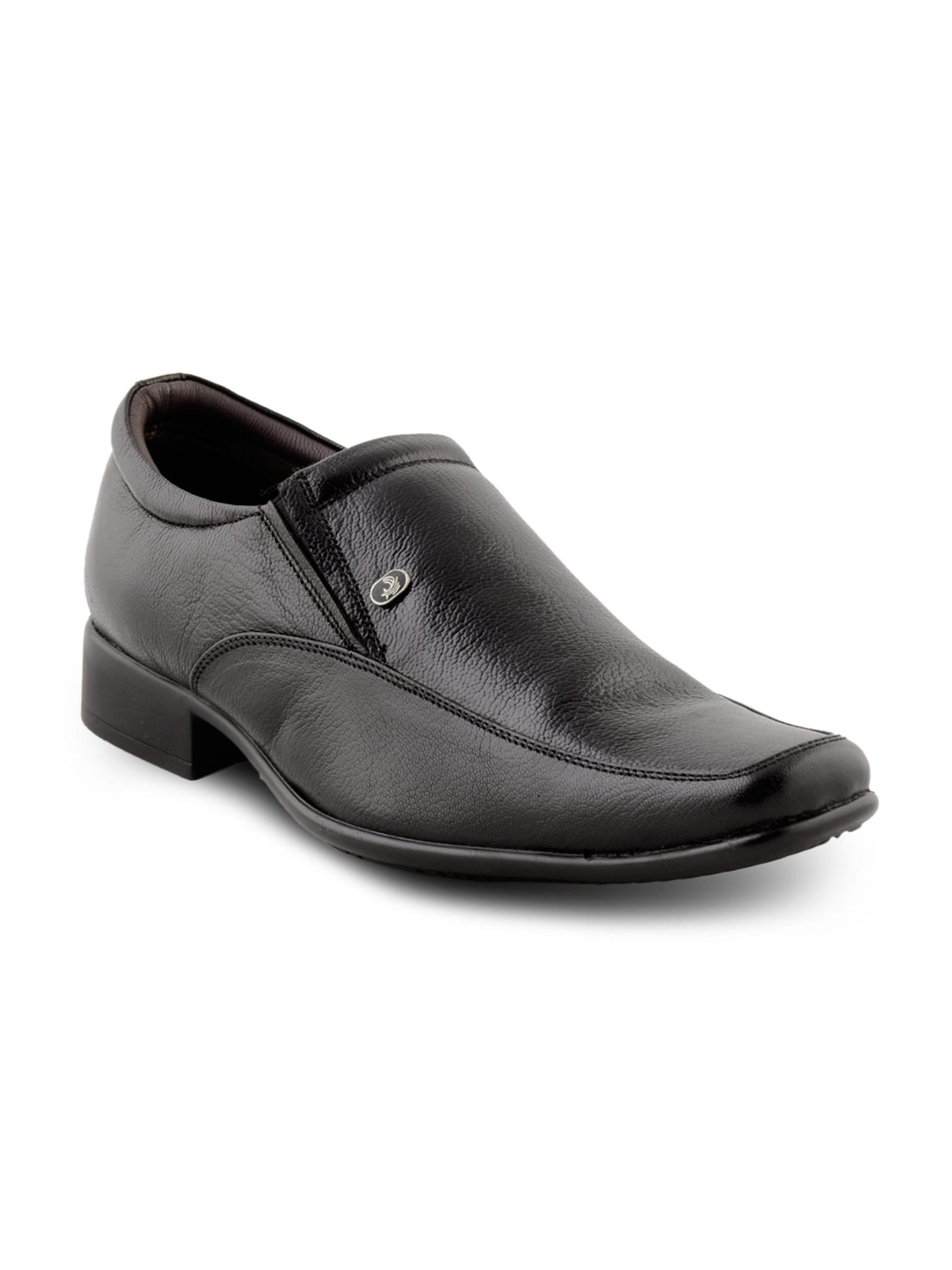
| Buckaroo men flores black formal shoes | men | formal shoes | black | formal | [] | nan | nan | 155 | buckaroo | 2 | 2.jpg |
| Gas men europa white shoes | men | casual shoes | white | casual | [] | nan | nan | 105 | gas | 3 | 3.jpg |
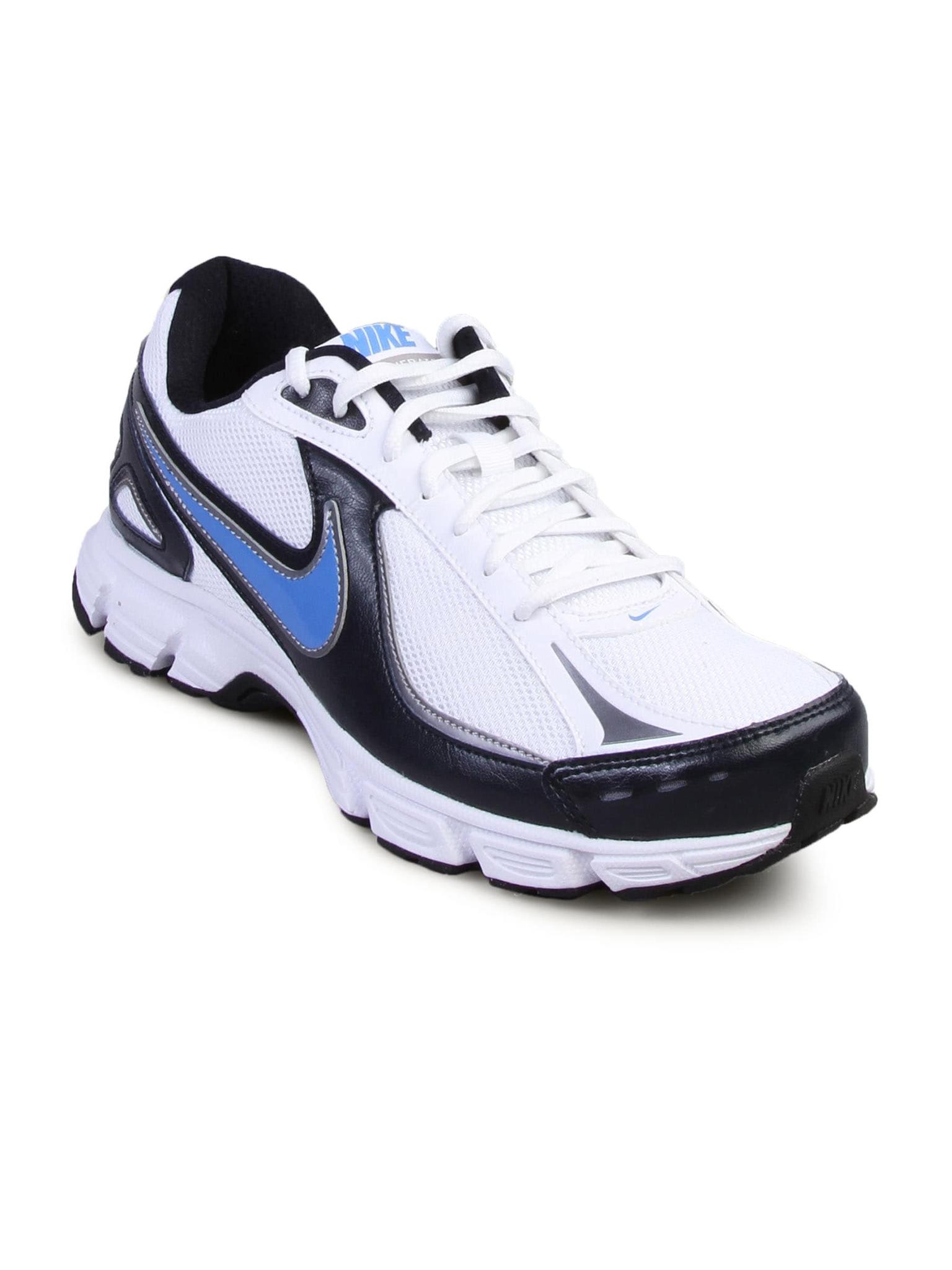
| Nike men's incinerate msl white blue shoe | men | sports shoes | white | sports | ['blue'] | nan | nan | 125 | nike | 4 | 4.jpg |
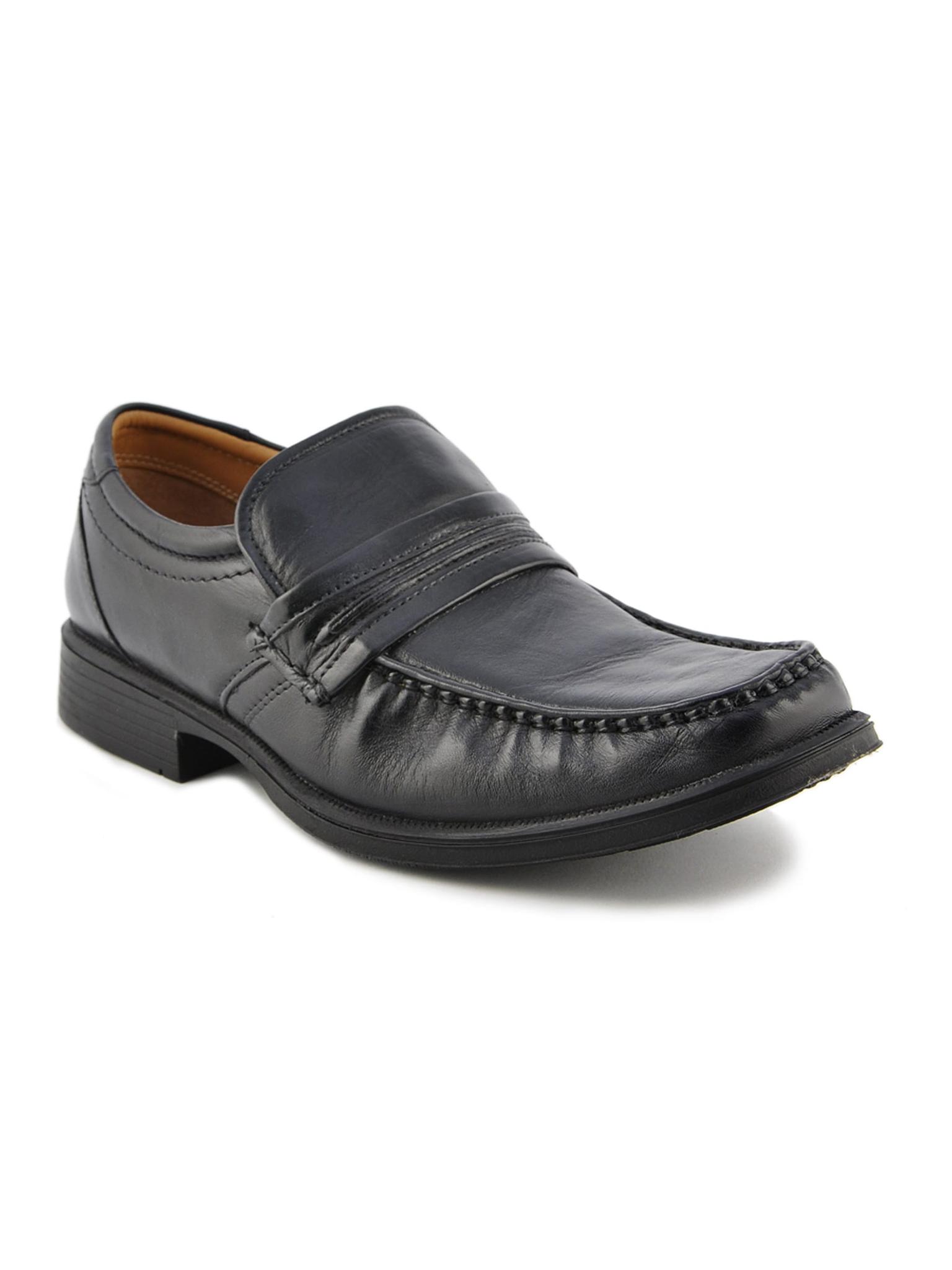
| Clarks men hang work leather black formal shoes | men | formal shoes | black | formal | [] | nan | nan | 220 | clarks | 5 | 5.jpg |
The shoe product data consists of 12 columns:
- product_title
- gender
- product_type
- color
- usage
- color_details
- heel_height
- heel_type
- price_usd
- brand
- product_id
- image
Next, let's display the product images for the first five shoes.
In a new cell, run:
width = 100
images_html = ""
image_data_path = 'data/footwear'
for img_file in df_shoes.head()['image']:
    img_path = os.path.join(image_data_path, img_file)
    # Add each image as an HTML <img> tag
    images_html += f'<img src="{img_path}" style="width:{width}px; margin-right:10px;">'
# Display all images in a row using HTML
display(HTML(f'<div style="display: flex; align-items: center;">{images_html}</div>'))
When you run this, you'll see a row of shoe images displayed in your Notebook:

Cost of vectorization
The next step is to vectorize the shoe product data:

We need to generate a vector, the numerical representation of each shoe in our shoe database
Before generating embeddings, let's quickly talk about tge cost of vectorizing the shoe data with AWS Bedrock and the AWS Titan multimodal model.
The charges depend on the number of text tokens and images processed.
Pricing details:
-
Text embeddings: $0.0008 per 1,000 input tokens
-
Image embeddings: $0.00006 per image
The provided SoleMates shoe dataset is fairly small, containing 1306 pair of shoes, making it affordable to vectorize.
For this dataset, I calculated the cost of vectorization and summarized the token counts below:
- Token count:
12746 tokens - Images:
1306 - Total cost:
~$0.09
Calculations:
(12746 tokens/1000)*0.0008 + (1306*0.00006) =
0.0885568
Optional: Using a pre-embedded dataset
This step is entirely optional and designed to accommodate various levels of access and resources.
If you prefer not to run the embedding process and generate embeddings or don't have access to AWS, you can use a pre-embedded dataset included in the repository.
This file contains all the embeddings and token counts, so you can follow this guide without additional costs.
This step is optional. For hands-on experience, I recommend generating the embeddings yourself to fully understand the workflow.
The pre-embedded dataset is located at:
data/solemates_shoe_directory_with_embeddings_token_count.csv
To load it in your Jupyter Notebook, use:
df_shoes_with_embeddings = pd.read_csv('data/solemates_shoe_directory_with_embeddings_token_count.csv')

# Convert string representations to actual lists
df_shoes_with_embeddings['titan_embedding'] = df_shoes_with_embeddings['titan_embedding'].apply(ast.literal_eval)
Using the pre-embedded dataset lets you skip the vectorization step and move directly to the next part of the guide.
This step is entirely optional and designed to accommodate various levels of access and resources.
For hands-on experience, I recommend running the embedding process to understand the workflow.
Let's get started with Amazon Bedrock in the next section.
Getting started with Amazon Bedrock
To use AWS Titan, you need access to Amazon Bedrock's foundation models.
Amazon Titan Multimodal Embeddings G1 model is a multimodal embedding model that converts both product texts and images into vectors.
Why use AWS Titan?
A multimodal model allows us to process a query like "red heels" and match it to not only product descriptions but also actual images of red heels in the database.
By combining text and image data, the model helps the AI agent provide more relevant and visually aligned recommendations based on the customer's input.

AWS Titan is a multimodal model, accepting images, text or both images and text
Follow these steps to request access to Amazon Bedrock.
1. Log in to AWS
Visit the AWS Management Console and sign in to your AWS account.
2. Navigate to AWS Bedrock
Use the search bar at the top of the AWS Management Console to search for "Bedrock":

3. Initiate access request
On the Amazon Bedrock service page, click Get Started:

In the popup, click Manage Model Access:

On the next page, click Manage Model Access again:

4. Selecting the models
In the model access section, select Amazon from the list of available models; this will check all the available models:

Selecting Amazon from the list of available models will grant you access to 5 models. For this guide, we'll use:
- Titan Multimodal Embeddings G1
- Titan Embeddings (optional)
- Titan Text - Lite (optional)
- Titan Text - Express (optional)
- Titan Image Generator (optional)
5. Finalize the Request
Scroll to the bottom of the page and click Request Model Access:

6. Confirmation
After requesting access, you will be redirected back to the Bedrock overview page. Here, your access status will be shown as pending or granted:

Once your access if confirmed, you'll be ready to set up the AWS Bedrock client in the next section.
Set up AWS Bedrock client
Let's initialize Amazon Bedrock runtime client so we can interact with AWS Titan to generate embeddings.
Add the following code snippet in a new Jupyter Notebook cell.
If you have a specific AWS profile, set it in the aws_profile variable; otherwise, leave it as None to use the default profile:
# Define your AWS profile
# Replace AWS_PROFILE with the name of your AWS CLI profile
# To use your default AWS profile, leave 'aws_profile' as None
aws_profile = os.environ.get('AWS_PROFILE')

# Specify the AWS region where Bedrock is available
aws_region_name = "us-east-1"

try:
    # Set the default session for the specified profile
    if aws_profile:
        boto3.setup_default_session(profile_name=aws_profile)
    else:
        boto3.setup_default_session()  # Use default AWS profile if none is specified

    # Initialize the Bedrock runtime client
    bedrock_runtime = boto3.client(
        service_name="bedrock-runtime",
        region_name=aws_region_name
    )
except NoCredentialsError:
    print("AWS credentials not found. Please configure your AWS profile.")
except Exception as e:
    print(f"An unexpected error occurred: {e}")
With the Bedrock client set up, you're ready to generate embeddings in the next section.
Generate product vectors
Now that your AWS Bedrock client is ready, it's time t generate product vectors.
In this next step, you'll add two new columns to your DataFrame:
titan_embedding: to store the embedding vectors generated by AWS Titantoken_count: to store the token count for each product title
Skip this step if you're using the pre-embedded dataset, as it already contains these columns.
Run this snippet in a new Jupyter Notebook cell to initialize the new columns:
# Initialize columns to store embeddings and token counts
df_shoes['titan_embedding'] = None  # Placeholder for embedding vectors
df_shoes['token_count'] = None  # Placeholder for token counts
Next, define a function to generate embeddings for each shoe.
This function reads each product's image and title, sends them to AWS Titan via the Bedrock runtime, and stores the resulting embedding and token count back into the DataFrame:
# Main function to generate image and text embeddings
def generate_embeddings(df, image_col='image', text_col='product_title', embedding_col='embedding', image_folder=None):

    if image_folder is None:
        raise ValueError("Please provide the path to the image folder.")

    for index, row in tqdm(df.iterrows(), total=df.shape[0], desc="Generating embeddings"):
        try:
            # Read and encode the image as base64
            image_path = os.path.join(image_folder, row[image_col])
            with open(image_path, 'rb') as img_file:
                image_base64 = base64.b64encode(img_file.read()).decode('utf-8')

            # Prepare input data for AWS Titan
            input_data = {"inputImage": image_base64, "inputText": row[text_col]}

            # Invoke the AWS Titan model via Bedrock runtime
            response = bedrock_runtime.invoke_model(
                body=json.dumps(input_data),
                modelId="amazon.titan-embed-image-v1",
                accept="application/json",
                contentType="application/json"
            )
            response_body = json.loads(response.get("body").read())

            # Extract embedding and token count from response
            embedding = response_body.get("embedding")
            token_count = response_body.get("inputTextTokenCount")

            # Validate and save the embedding and token count
            if isinstance(embedding, list):
                df.at[index, embedding_col] = embedding  # Save embedding as a list
                df.at[index, 'token_count'] = int(token_count)  # Save token count as an integer
            else:
                raise ValueError("Unexpected response: embedding is not a list.")

        except Exception as e:
            print(f"Error for row {index}: {e}")
            df.at[index, embedding_col] = None  # Handle errors gracefully

    return df
What the function does
The generate_embeddings function:
- Reads each product's image file and encodes it as base64
- Combines the encoded image and product title into a JSON payload
- Calls AWS Titan via Amazon Bedrock to generate an embedding vector
- Extracts the embedding and token count from the response
- Stores the results back into the DataFrame
Parameters
df: The DataFrame containing the dataimage_col: Column name in the DataFrame where image filenames are stored (default:'image')text_col: Column name in the DataFrame where text data (like product titles) is stored (default:'product_title')embedding_col: Column name where embeddings will be stored (default:'embedding')image_folder: The folder path where images are located (required)
When you've added this function, run this next cell to start generating embeddings.
Running this next function will start generating vectors by calling Amazon Bedrock, incurring a cost of approximately $0.09.
It may take around 10 minutes to process all 1306 pairs of shoes
Run the following cell to start generating embeddings:
# Generate embeddings for the product data
df_shoes = generate_embeddings(
    df=df_shoes,
    embedding_col='titan_embedding',
    image_folder='data/footwear'
)
A progress bar will display the process.
It takes approximately 10 minutes to generate embeddings for the 1306 pair of shoes in our shoe database.

The vectorization of 1306 shoes takes approximately 10 minutes
Once all embeddings are generated, save your updated DataFrame to a CSV file to avoid having to re-run the process:
# Save the dataset with generated embeddings to a new CSV file
# Get today's date in YYYY_MM_DD format
today = datetime.now().strftime('%Y_%m_%d')

# Save the dataset with generated embeddings to a CSV file
df_shoes.to_csv(f'shoes_with_embeddings_token_{today}.csv', index=False)
print(f"Dataset with embeddings saved as 'shoes_with_embeddings_token_{today}.csv'")
This CSV file will include your product data along with a 1024-length vector for each product title and the corresponding token count.
Querying the vectorized data
Now that your dataset contains embeddings, we can implement a simple vector similarity search to find the products most relevant to a query.
In this section, you'll:
- Generate a query embedding for a text query (e.g. "red shoes")
- Calculate similarity scores between the query and product embeddings using both cosine similarity and dot product
- Retrieve and visualize the top matching products
Testing Vectorization vs. Production Search
In this guide, we use cosine similarity and dot product similarity as simple ways to test whether our vectorized product data makes sense. These methods help validate that the embeddings correctly capture relationships between products.
However, in real-world applications, vectors are typically stored in vector databases (such as Pinecone, Weaviate, or FAISS) that handle similarity search efficiently at scale. A follow-up guide will cover how to upsert these vectors into a database and optimize retrieval for production-ready AI-powered search and recommendations.
What is cosine similarity?
Cosine similarity measures how close two vectors are by calculating the cosine of the angle between them in a multi-dimensional space.

Simplifying Search with Cosine Similarity
Using cosine similarity, we can compare a customer's search query in vector form against all product vectors in our database to rank products. The closer a product's vector is to the query vector, indicated by a higher cosine score, the higher it ranks as a match to the customer's needs.
Example: red yoga pants
Let's say a customer searches for red yoga pants. Cosine similarity helps our search algorithm prioritize red yoga pants by recognizing their vector is closer (has a higher cosine similarity score) to the customer's query vector:

In contrast, a less similar product, like yellow yoga pants, has a wider angle to the query vector, resulting in a lower similarity score:

Let's start by vectorizing an input query like "red shoes" and try to retrieve the closest matching products.
1. Define helper functions
a. Request AWS Titan embeddings
Define a helper function that sends a text, or image (or both), input to AWS Titan and returns its embedding vector.
Add this function to a new cell in your Jupyter Notebook:
def request_embedding(image_base64=None, text_description=None):
    """
    Request embeddings from AWS Titan multimodal model.

    Parameters:
        image_base64 (str, optional): Base64 encoded image string.
        text_description (str, optional): Text description.

    Returns:
        list: Embedding vector.
    """
    input_data = {"inputImage": image_base64, "inputText": text_description}
    body = json.dumps(input_data)

    # Invoke the Titan multimodal model
    response = bedrock_runtime.invoke_model(
        body=body,
        modelId="amazon.titan-embed-image-v1",
        accept="application/json",
        contentType="application/json"
    )

    response_body = json.loads(response.get("body").read())

    if response_body.get("message"):
        raise ValueError(f"Embeddings generation error: {response_body.get('message')}")

    return response_body.get("embedding")
b. Cosine similarity function
Next, we'll need functions for calculating similarities between the input query and our shoes.
This function computes cosine similarity scores between the query vector and each product embedding:
def compute_cosine_similarities(query_vec, embeddings):
    """
    Compute cosine similarities between a query vector and a list of embeddings.

    Parameters:
        query_vec (list or np.array): Query embedding vector.
        embeddings (list of lists): List of product embedding vectors.

    Returns:
        np.array: Array of cosine similarity scores.
    """
    # Convert lists to NumPy arrays
    query_vec = np.array(query_vec).reshape(1, -1)
    embeddings = np.array(embeddings)
    return cosine_similarity(query_vec, embeddings).flatten()
c. Dot product similarity function
This function computes dot product similarity scores:
def compute_dot_product_similarity(query_vec, embeddings):
    """
    Compute dot product similarities between a query vector and a list of embeddings.

    Parameters:
        query_vec (list or np.array): The query embedding vector.
        embeddings (list of lists): List of product embedding vectors.

    Returns:
        np.array: Array of dot product similarity scores.
    """
    query_vec = np.array(query_vec).flatten()  # Ensure query is a 1D array
    embeddings = np.array(embeddings)
    # Compute dot product similarity for each embedding
    return np.dot(embeddings, query_vec)
2. Query your data
We're ready to query our vectors.
a. Prepare the product embeddings
Start by extracting a list of our dense (AWS Titan) product vectors from your DataFrame:
product_embeddings = df_shoes['titan_embedding'].tolist()
b. Generate a query embedding
Then, let's vectorize the input query "red shoes":
customer_query = "red heels"
query_embedding = request_embedding(text_description=customer_query)
c. Compute similarities
Calculate both cosine and dot product similarities between the query and product embeddings:
cosine_similarities = compute_cosine_similarities(query_embedding, product_embeddings)
dot_similarities = compute_dot_product_similarity(query_embedding, product_embeddings)
d. Retrieve top matching products
Select the top N similar products based on each similarity measure.
Here, num_neighbors is set to 6, but you can adjust this number as needed:
num_neighbors = 6  # Change this to the desired number of neighbors
top_indices_cosine = np.argsort(cosine_similarities)[::-1][:num_neighbors]
top_indices_dot = np.argsort(dot_similarities)[::-1][:num_neighbors]
3. Visualize the results
We have our products, finally let's visualize them.
Use the helper function below to display the matching products:
def visualize_neighbors(df, neighbor_indices, image_data_path='data/footwear', width=100):
    """
    Visualize the neighbor products from the cosine similarity search.

    Parameters:
        df (pd.DataFrame): DataFrame containing product data.
        neighbor_indices (list): List of indices for the neighbor products.
        image_data_path (str): Folder path where product images are stored.
        width (int): Display width of each image in pixels.
    """
    images_html = ""
    for idx in neighbor_indices:
        product = df.iloc[idx]
        img_file = product['image']
        product_title = product['product_title']
        img_path = os.path.join(image_data_path, img_file)
        images_html += (
            f'<div style="margin-right:10px; text-align:center;">'
            f'<img src="{img_path}" style="width:{width}px;"><br>'
            f'<span>{product_title}</span>'
            f'</div>'
        )
    display(HTML(f'<div style="display: flex; align-items: center;">{images_html}</div>'))
Now, run this code in a new cell to visualize the top neighbors for both similarity methods:
# Example usage: Visualize top 5 neighbors (using the indices from the cosine similarity search)
visualize_neighbors(df_shoes, top_indices_cosine, image_data_path='data/footwear', width=100)

# Example usage: Visualize top 5 neighbors (using the indices from the cosine similarity search)
visualize_neighbors(df_shoes, top_indices_dot, image_data_path='data/footwear', width=100)
You should see the top matching products for the input query "red heels":
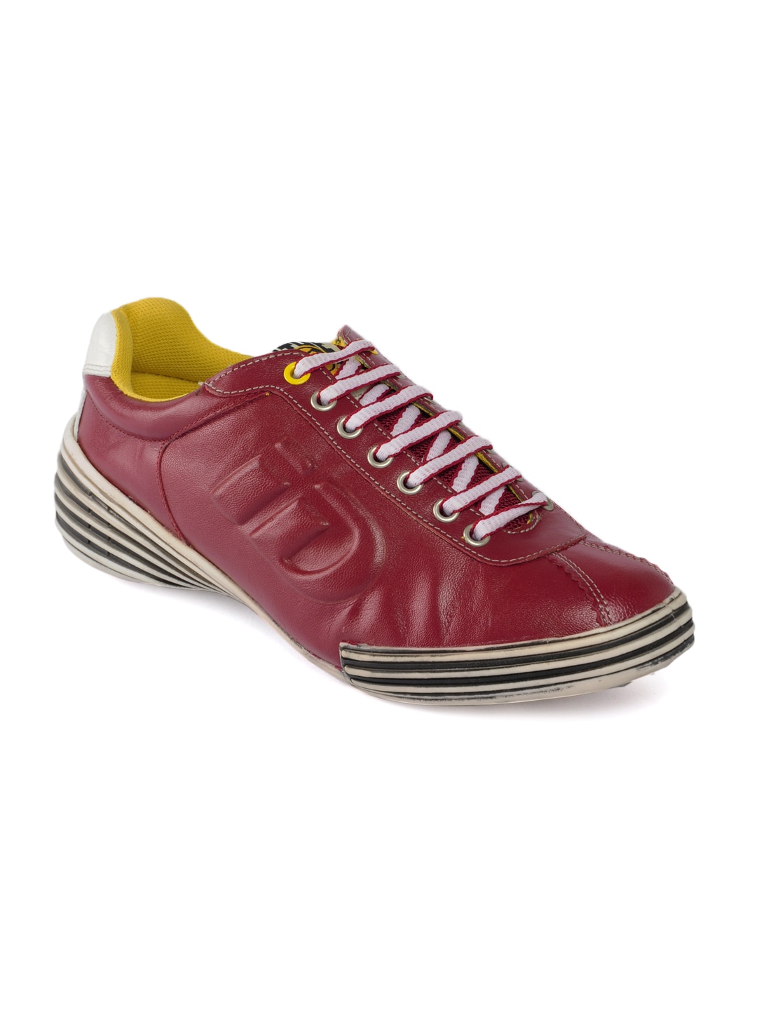
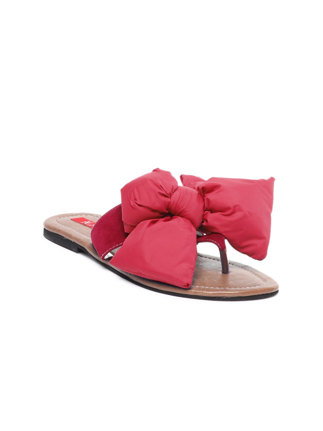

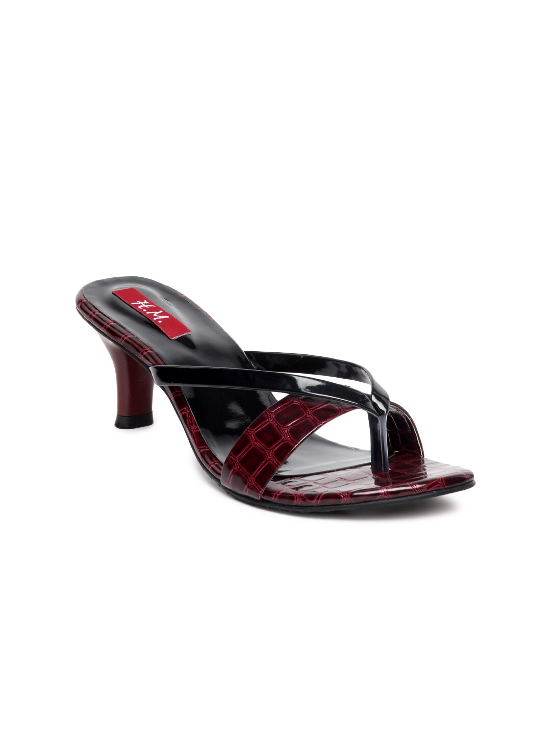
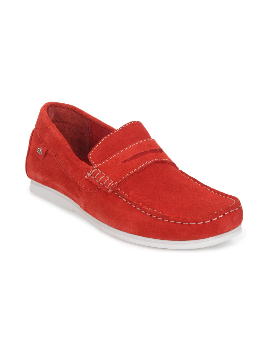
In this example, both cosine and dot product methods returned the same products.
4. Try another query
Great, our vectors and vector query works, let's try one more query: "blue shoes":
customer_query = "blue shoes"
query_embedding = request_embedding(text_description=customer_query)
cosine_similarities = compute_cosine_similarities(query_embedding, product_embeddings)
dot_similarities = compute_dot_product_similarity(query_embedding, product_embeddings)
num_neighbors = 6  # Change this to the desired number of neighbors
top_indices_cosine = np.argsort(cosine_similarities)[::-1][:num_neighbors]
top_indices_dot = np.argsort(dot_similarities)[::-1][:num_neighbors]

# Visualize top 5 neighbors (using the indices from the cosine similarity search)
visualize_neighbors(df_shoes, top_indices_cosine, image_data_path='data/footwear', width=100)

# Visualize top 5 neighbors (using the indices from the dot product similarity search)
visualize_neighbors(df_shoes, top_indices_dot, image_data_path='data/footwear', width=100)
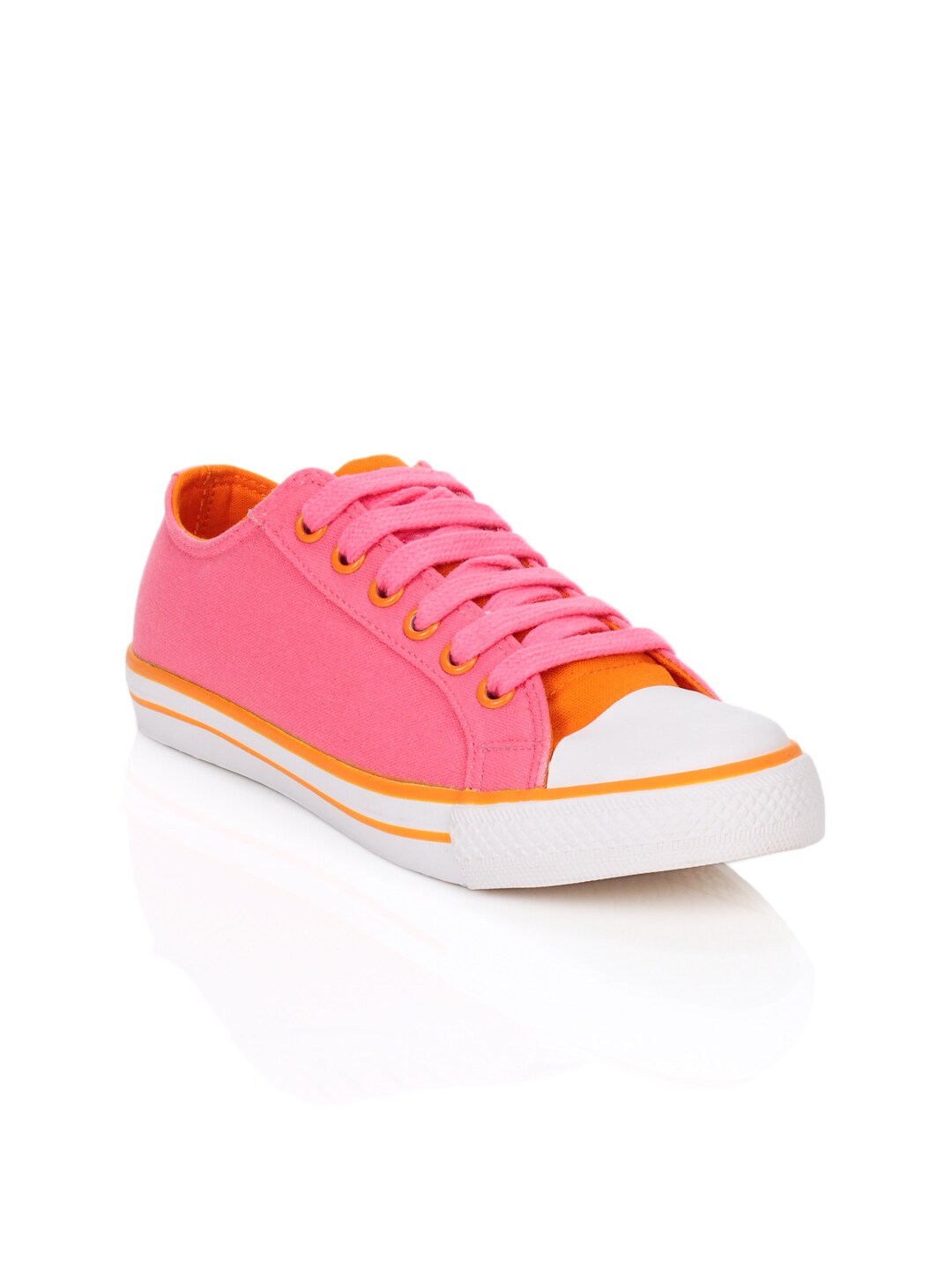
You should see these 6 shoes:
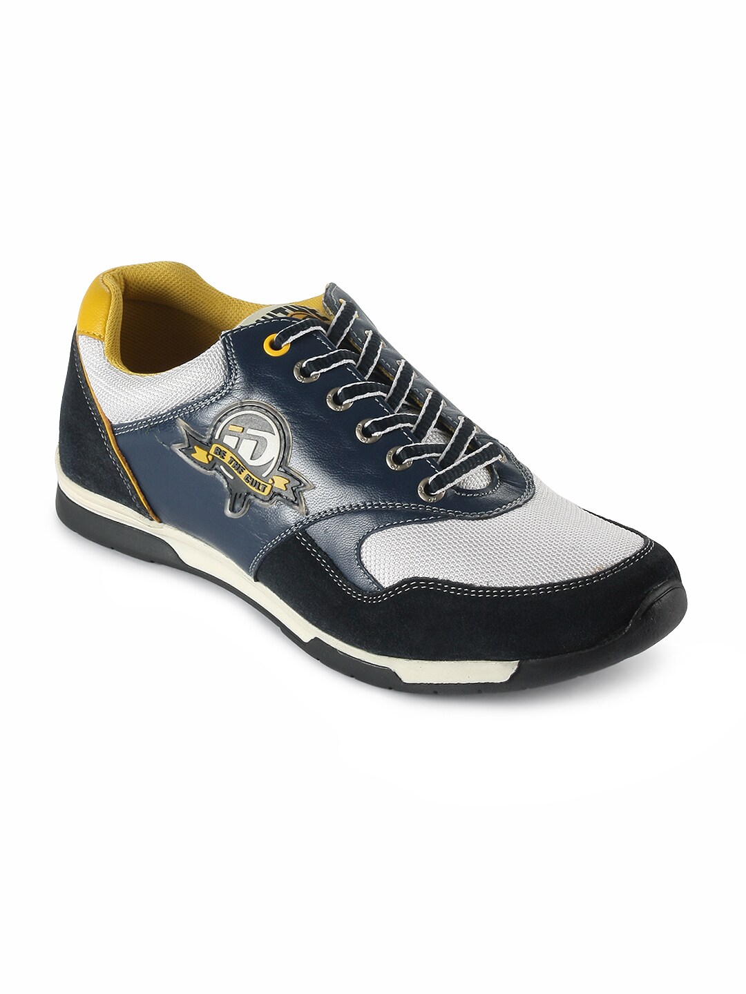
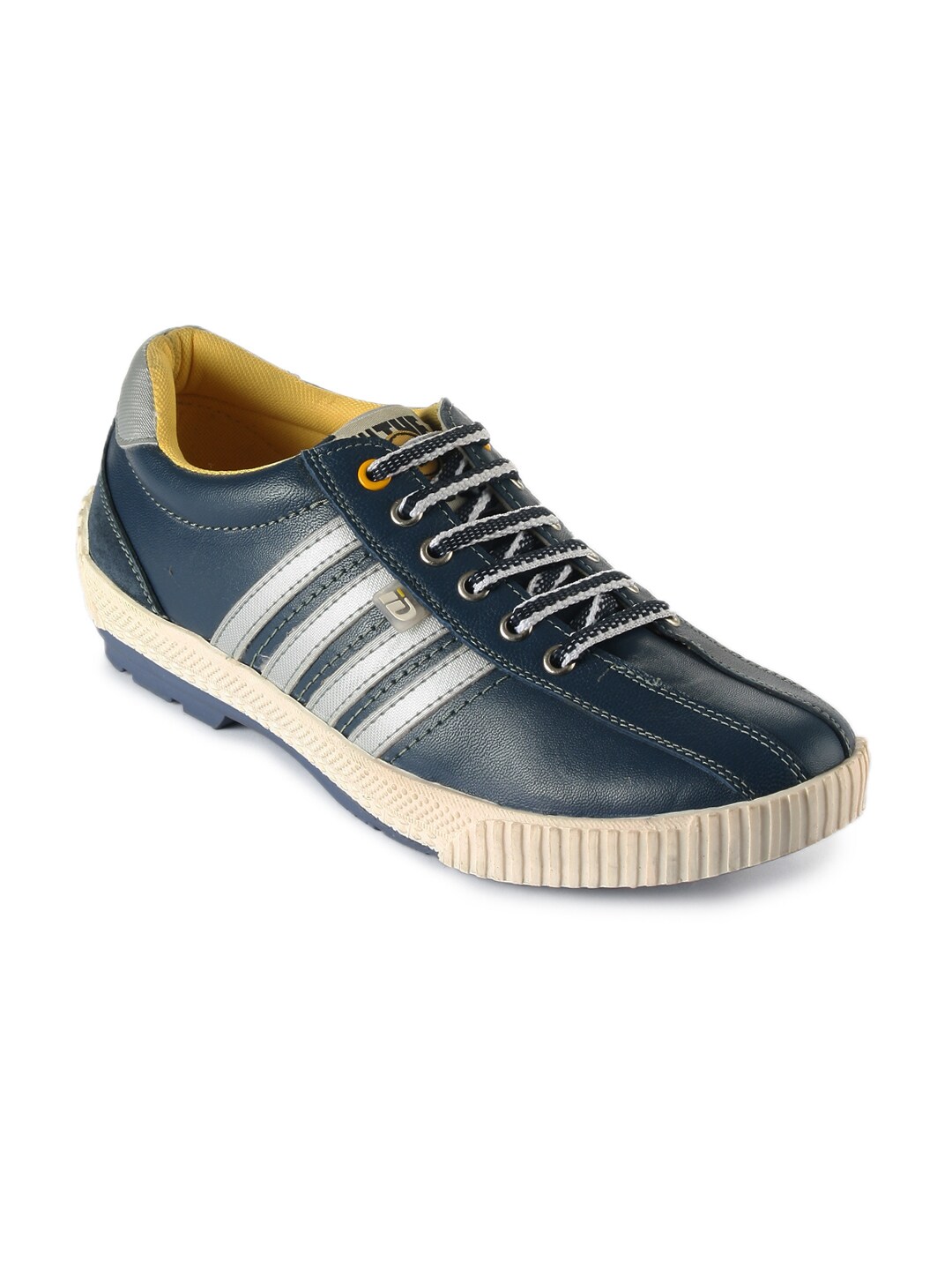
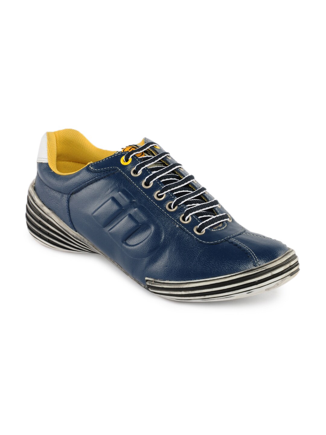
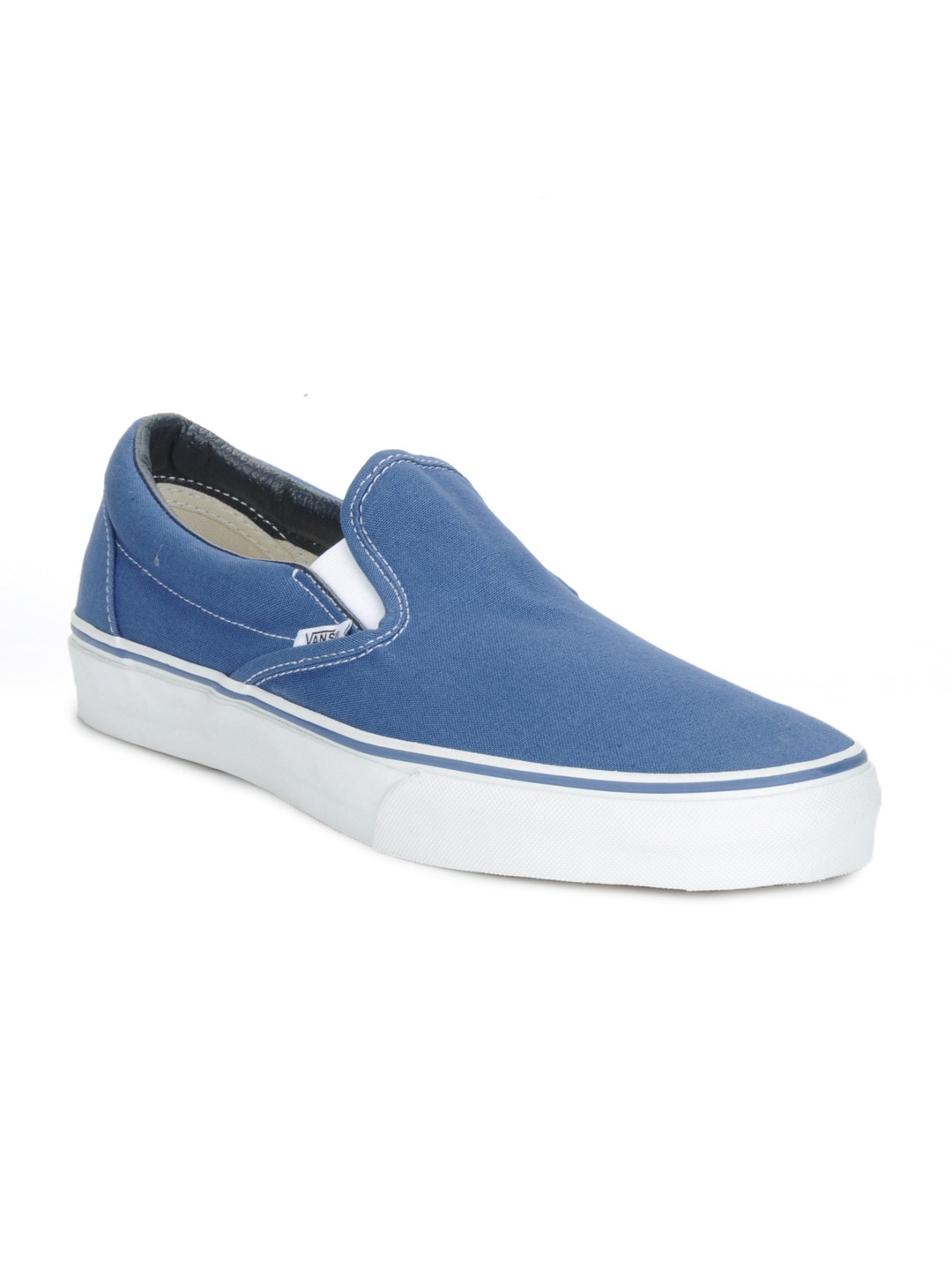
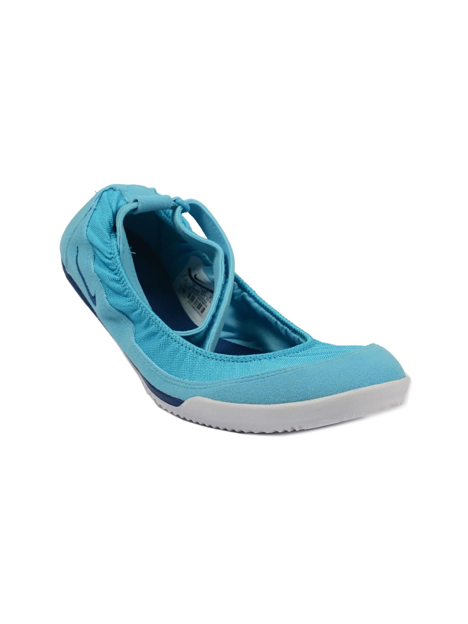
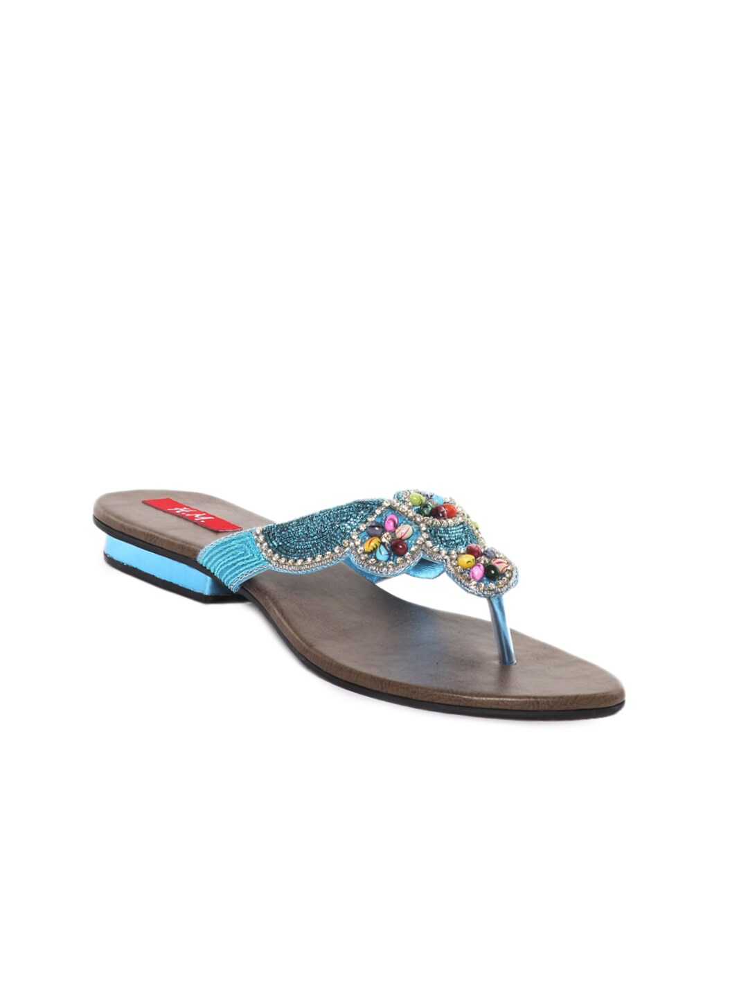
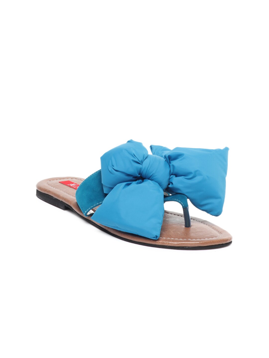
You might notice a slight difference in the ranking for "blue shoes", illustrating how the two similarity metrics can sometimes produce different results.
Comparison of similarity metrics
Here's a structured comparison of cosine similarity and dot product similarity:
| Feature | Cosine Similarity | Dot Product Similarity |
|---|---|---|
| Definition | Measures the cosine of the angle between vectors | Measures the sum of element-wise multiplication |
| Scale Sensitivity | Not affected by vector magnitude | Affected by vector magnitude |
Summary
In this guide, we covered:
1. Setting up:
- Installing dependencies, loading the SoleMates dataset, and initializing the AWS Bedrock client
2. Vectorizing data:
- Generating embeddings for both product images and titles using AWS Titan
3. Multimodal models:
- Understanding the benefits of multimodal models like AWS Titan for combining text and image data
4. Querying vectors:
- Creating helper functions to generate query embeddings and retrieving the closest product matches using both cosine similarity and dot product
These steps provide a solid foundation for using vectorization to enhance e-commerce search and recommendations.
Next Steps
Now that you've built a vector search solution with AWS Titan, here are some ideas to take your project even further:
-
Integrate and experiment:
Embed your vector search into your e-commerce platform and try out different similarity metrics (cosine vs. dot product) to fine-tune your recommendations -
Scale your solution:
As your product database grows, consider exploring specialized vector search libraries like FAISS or Pinecone for improved performance -
Learn More and Level Up:
Ready to build an AI agent that handles complex, multi-color product queries? Check out my free mini-course "How to Build an AI Agent to Handle Multi-Color Product Queries":
In this step-by-step mini-course, you'll learn how to create an AI agent in Jupyter Notebook using Python, Pinecone, and LlamaIndex - no deployment required. You'll get hands-on experience building a smarter query engine that goes beyond basic retrieval.
By following these next steps, you'll be well on your way to creating advanced, AI-powered search and recommendation systems.
Download the Notebook
To follow along or revisit the complete code walkthrough for this guide, download the Jupyter Notebook file:
Download vectorizing_ecommerce_data_aws_titan.ipynb ↗
This notebook contains all the code snippets and instructions from the guide.