Using Jupyter Agent for data exploration: a practical guide

Jupyter Agent automates Jupyter Notebook creation, making it easy to analyze datasets before vectorizing them for Retrieval-Augmented Generation (RAG).

In this guide, we'll use Jupyter Agent Hugging Face space to explore a fictional shoe store's dataset, uncover key insights, and prepare the data for an AI-powered search system.

The first step of a simple RAG system is data exploration. However, this crucial step is often overlooked, even though the quality of the data directly impacts retrieval results.

Let's explore how we can use Jupyter Agent to analyze product data before vectorizing it for a RAG system.

Overview

What we'll cover:

1. What Jupyter Agent is
2. Why data exploration matters
3. How to use Jupyter Agent for data exploration

What is Jupyter Agent?

Jupyter Agent is a Hugging Face space ↗ that lets an LLM generate and execute code inside a Jupyter Notebook.

Instead of manually writing scripts, you can upload a dataset, enter a structured prompt, and let the AI generate a working notebook:

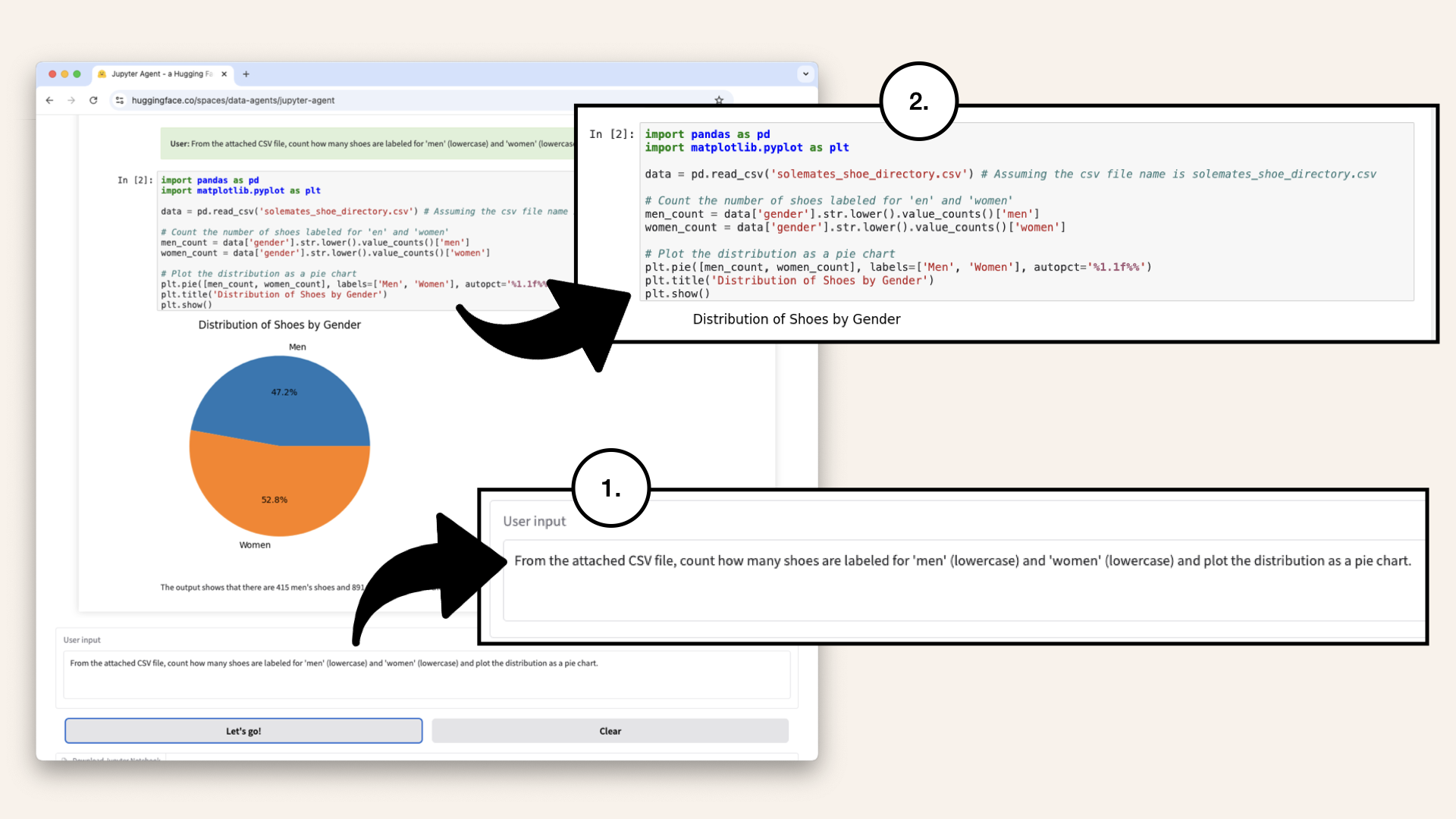
Choose an LLM, enter a prompt, and the chosen model generates an entire notebook

Jupyter Agent is an AI-powered assistant for Jupyter Notebooks.

It can:

✅ Load and explore datasets
✅ Execute Python code
✅ Generate charts and plots
✅ Follow step-by-step instructions

The LLM outputs code cells, which you can download as a complete Jupyter Notebook:

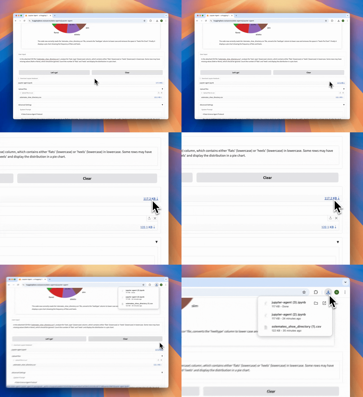
You can download the LLM output as a complete Jupyter Notebook

Use case: data exploration

The first step in building a RAG system is acquiring and understanding the data:

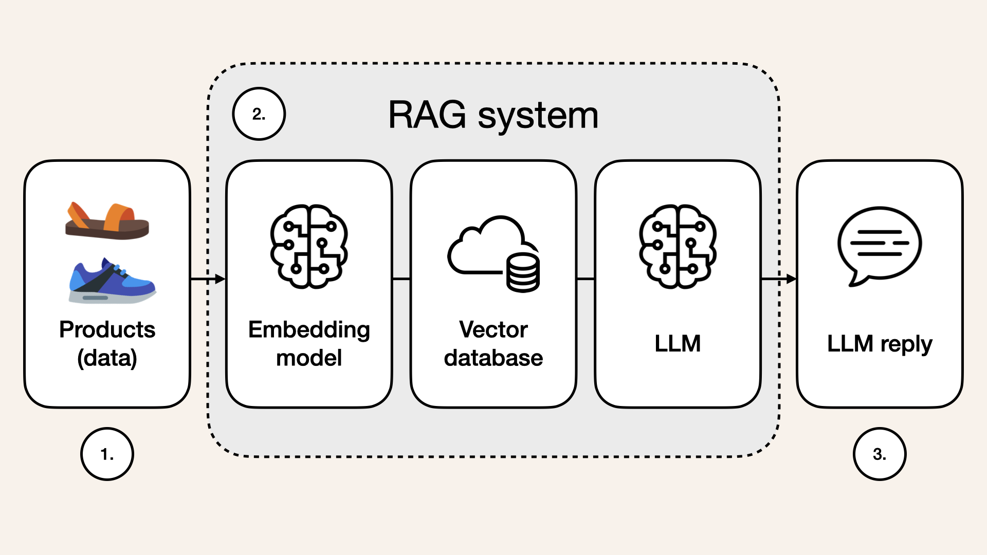
Overview of a simple RAG system, starting with data, then embedding model, followed by a vector database and finally an LLM response

Many skip the data exploration step, assuming any structured dataset will work for retrieval. But without a clear understanding of column distributions, missing values, and data consistency, retrieval quality suffers.

Let's use Jupyter Agent to analyze product data for our fictional shoe store, SoleMates:

SoleMates is our fictional online shoe store

For example, if we don't check our SoleMates dataset, we might not realize that some shoe colors are mislabeled (e.g., 'dark blue' vs. 'navy'), leading to inaccurate search results. Jupyter Agent helps us catch these issues early, ensuring our AI system retrieves the right products instead of showing incomplete or irrelevant results.

This guide focuses on that crucial first step - before designing or building a RAG system - where we analyze the data itself.

Instead of jumping straight into embeddings and retrieval, we first need to ensure our dataset is clean, structured, and ready for use:

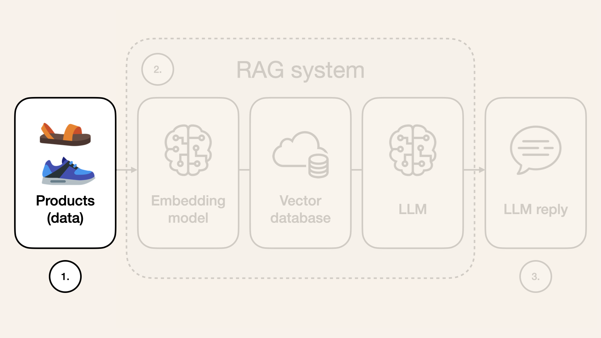
This guide focuses on that crucial first step - before designing or building a RAG system

How to use Jupyter Agent for data exploration

Step 1: Upload the dataset

Visit the jupyter-agent Hugging Face space:

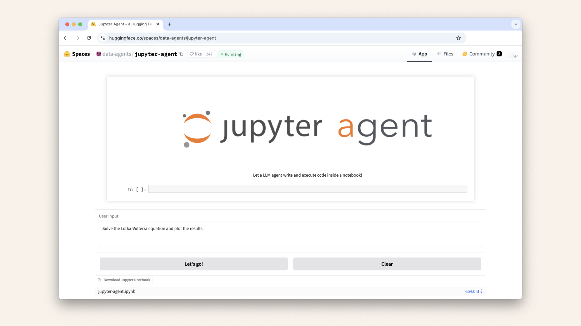
Visit the jupyter-agent Hugging Face space

Before we type our input, let's download the SoleMates product dataset. I've prepared a CSV file with product details such as product titles, colors and brands.

Download this CSV: SoleMates shoe product data ↗

Once downloaded, expand the Upload files tab and upload the CSV file with SoleMates product data:

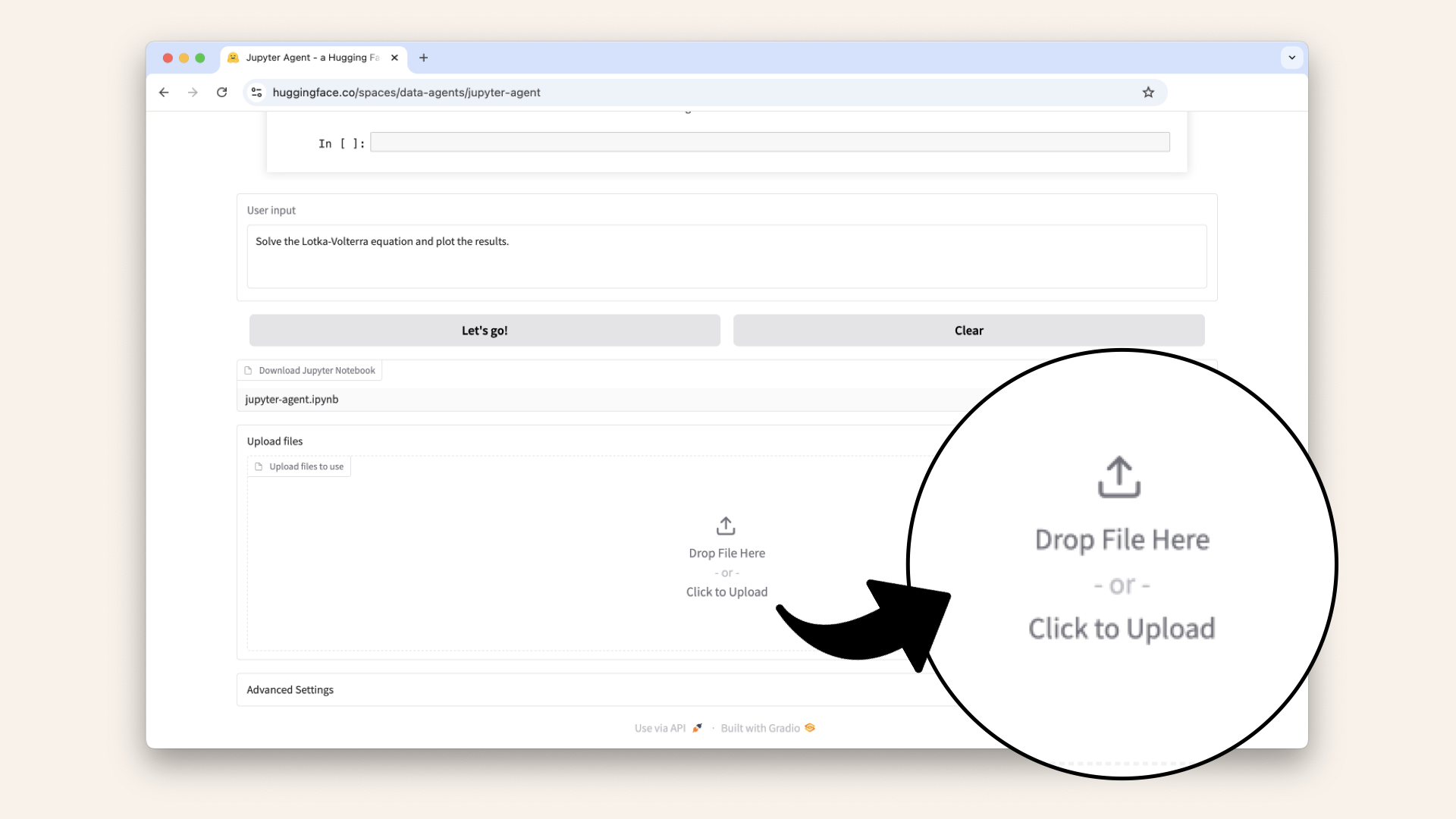
Upload the CSV file with SoleMates product data

Step 2: Select an LLM

Expand the Advanced Settings and select an LLM.

For this guide I'll go with meta-llama/Llama-3.1-70B-Instruct:

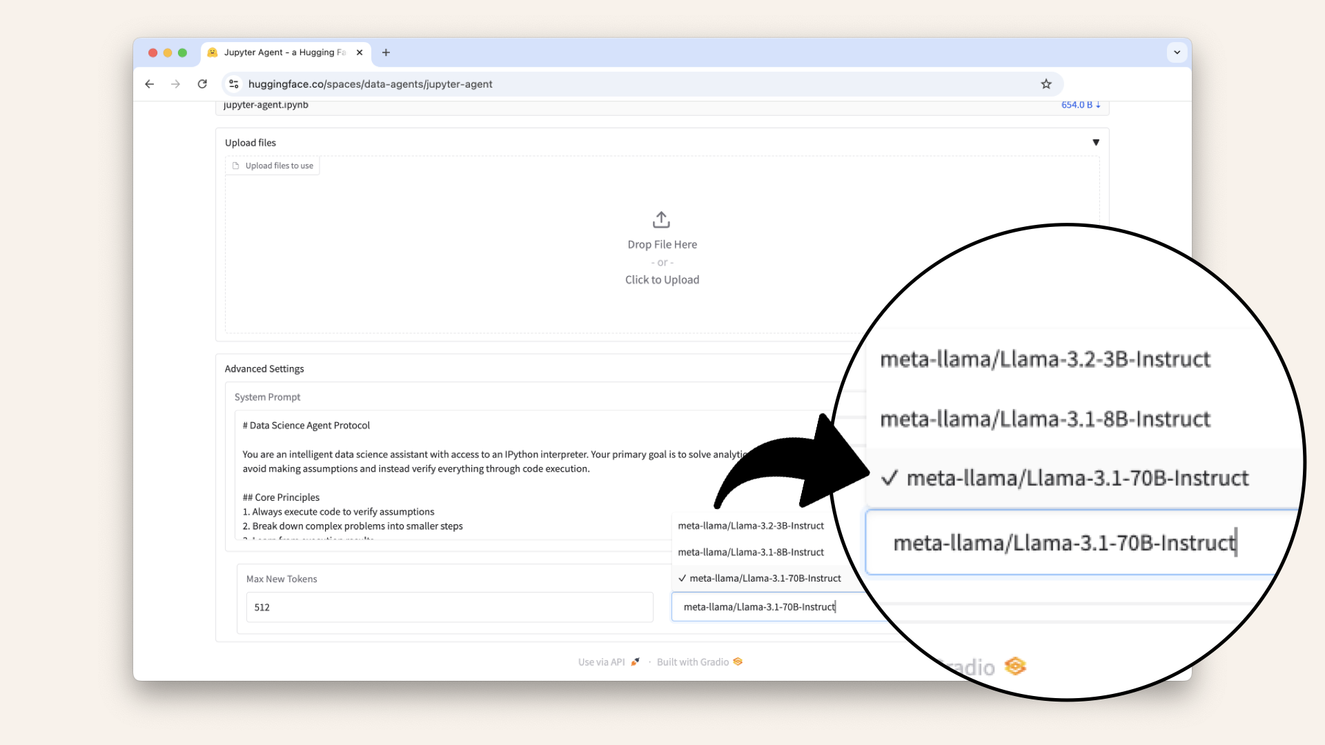
Expand the Advanced Settings and select an LLM

Supported Models

Jupyter Agent Hugging Face Space ↗ supports multiple models, each suited for different types of analysis:

• meta-llama/Llama-3.1-8B-Instruct - For general-purpose data exploration
• meta-llama/Llama-3.2-3B-Instruct - A lightweight option for quick computations
• meta-llama/Llama-3.1-70B-Instruct - Best for handling complex tasks and large datasets

Step 3: Start exploring the data

Now, let's start to explore the data. Let's start by having a look at the available categories.

Exploring the data

Check data structure

Type the following in the User input field and click Let's go! to ask the model to analyze our data:

Type the following in the User input field

Load the attached CSV file and describe its structure. List all column names, data types, and the number of rows.

This will prompt the LLM to read the CSV file we uploaded and start to explore the data:

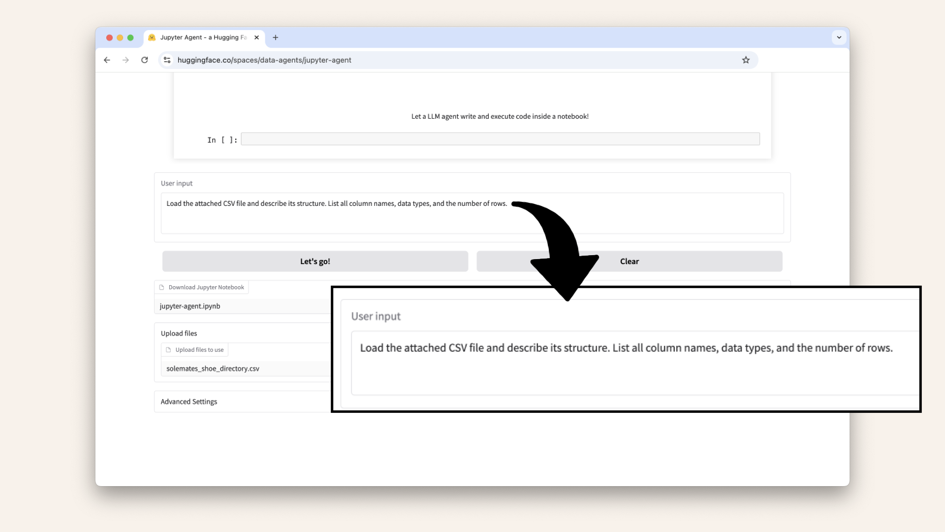
Add the first prompt to the User input field and click Let's go!

Expected output: The LLM reads the CSV and displays an overview of columns, their types, and row count.

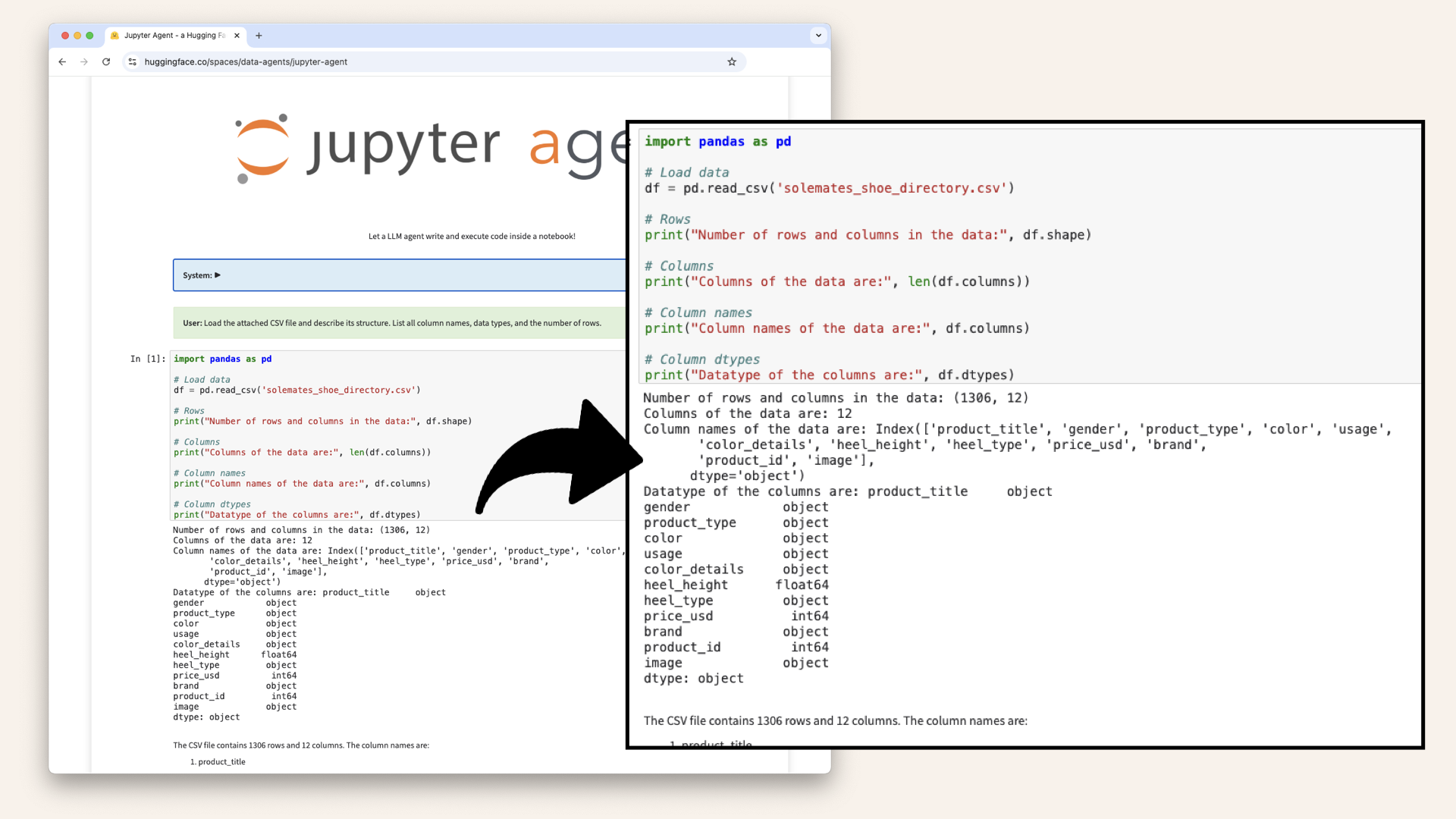
Run the prompt and this will generate an overview of the dataset

Your LLM reply might look different

The LLM responses are nondeterministic but you should see some kind of generated overview of the dataset.

If you scroll further down you should also see an overview of the column names and data types:

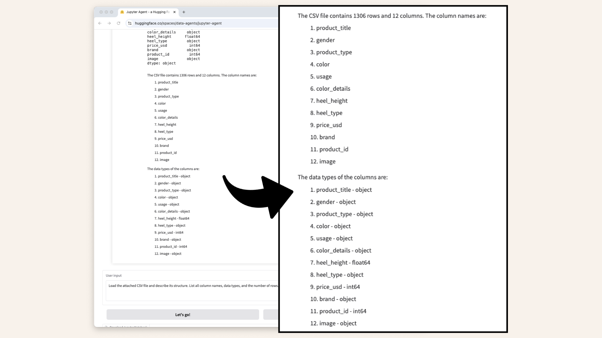
The LLM generated an overview of the column names and data types

Plot men's vs. women's shoes

Next, let's analyze gender distribution.

Type the following in the User input field and click Let's go! again:

Type the following in the User input field

From the attached CSV file, count how many shoes are labeled for 'men' (lowercase) and 'women' (lowercase) and plot the distribution as a pie chart.

Expected output: A pie chart showing the proportion of men's and women's shoes:

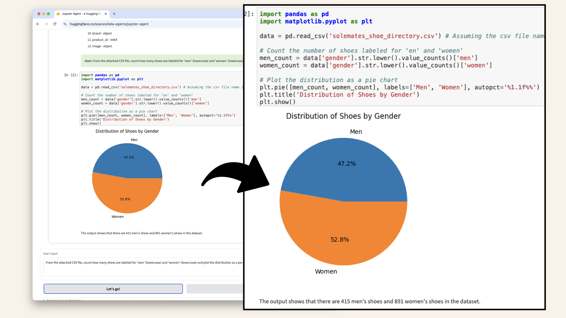
The LLM analyzes gender distribution

Identify the most common colors

Let's also analyze color trends.

Type this prompt into the User input field and click Let's go!:

Type the following in the User input field

From the attached CSV file ('solemates_shoe_directory.csv'), find the five most common colors in the 'color' (lowercase) column. The 'color' column contains color names as text (e.g., 'black', 'white', 'red'), not hex codes. Display these five colors in a bar chart, with the color names on the x-axis and their count on the y-axis.

Expected output: A bar chart visualizing the most common shoe colors:

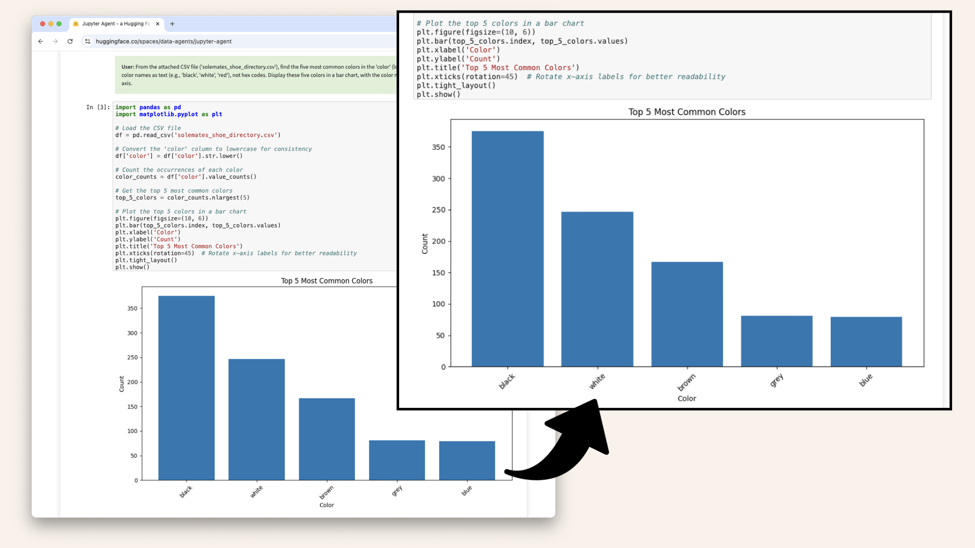
The LLM generates a bar chart of the top 5 most common shoe colors in the dataset

Compare flats vs. heels

Looking back at the first prompt where we checked the data structure, we're seeing a column named 'heel_type':

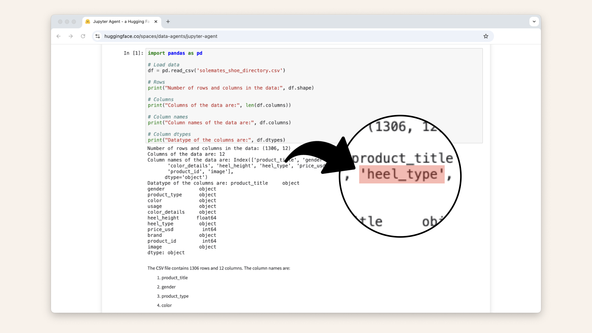
The previous data structure analysis showed a columned named heel_type

Let's write a prompt that plots the different heel types.

Add the following to the User input field and click Let's go!;

Type the following in the User input field

In the attached CSV file ('solemates_shoe_directory.csv'), analyze the 'heel_type' (lowercase) column, which contains either 'flats' (lowercase) or 'heels' (lowercase). Some rows may have missing values (NaN or None), which should be ignored. Count the number of 'flats' and 'heels' and display the distribution in a pie chart.

This generates a new pie chart with the distribution of heel types:

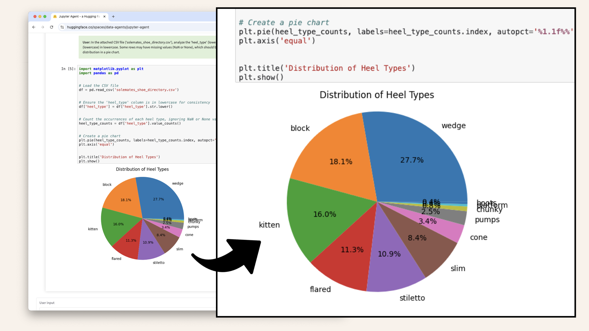
The LLM generates a new pie chart with heel type distribution

Download the generated notebook

Once the LLM has generated the code, you can download the Jupyter Notebook file, ready to run locally or modify as needed:

You can download the LLM output as a complete Jupyter Notebook

Conclusion

Jupyter Agent make it easy to automate Jupyter Notebook creation and quickly explore datasets.

Instead of manually writing pandas scripts, you can upload a dataset, ask a few well-defined prompts, and get structured insights within minutes.

I've downloaded the final Jupyter Notebook - ready to run and modify.

Here it is: Final data exploration Jupyter Notebook ↗

Try it out yourself and see how Jupyter Agent can streamline your workflow.

Try it here: Jupyter Agent Hugging Face Space ↗

---

Want to build your own AI agent? 🎯

If you're interested in AI-powered search and recommendation systems, check out my free mini-course:

Build an AI Agent for Multi-Color Product Queries

In this step-by-step course, you'll:

✅ Vectorize product data using AWS Titan
✅ Query a vector database with Pinecone and LlamaIndex
✅ Build an AI agent that filters by multiple colors & attributes
✅ Work entirely in Jupyter Notebook - no deployment needed

Join for free and start building today!