How to build an AI agent with LlamaIndex that can handle multiple color requirements

January 20, 2025 · 48 min read

AI Consultant

When an e-commerce customer asks for something like women's black shoes with red details, naive chatbots often struggle to apply multiple color filters simultaneously.

In this post, learn how to build a more advanced AI agent using Python, Pinecone and LlamaIndex, complete with metadata filtering and real-world code examples to handle multi-color product queries seamlessly.

Introduction

This is a step-by-step guide on how to build an AI agent with LlamaIndex that can handle multiple color requirements, like when a customer asks "I need women's black shoes with red details".

We'll use a made-up online shoe store to illustrate how a simple or naive chatbot handles the request and then we'll build an AI agent from scratch to show how the AI agent tackles the same challenge.

Prerequisites

We'll use Python and Jupyter Notebook throughout this walkthrough and I've prepared a dataset with product data and a folder with shoe images.

We'll use AWS Titan multimodal model to generate embeddings and finally upsert our vectors to cloud-based vector database Pinecone.

Introducing SoleMates

SoleMates is our fictional online shoe store we'll use to illustrate these concepts throughout this guide:

SoleMates is our fictional online shoe store

Challenge: handling multi-color queries

Scenario

A customer asks your simple RAG system:

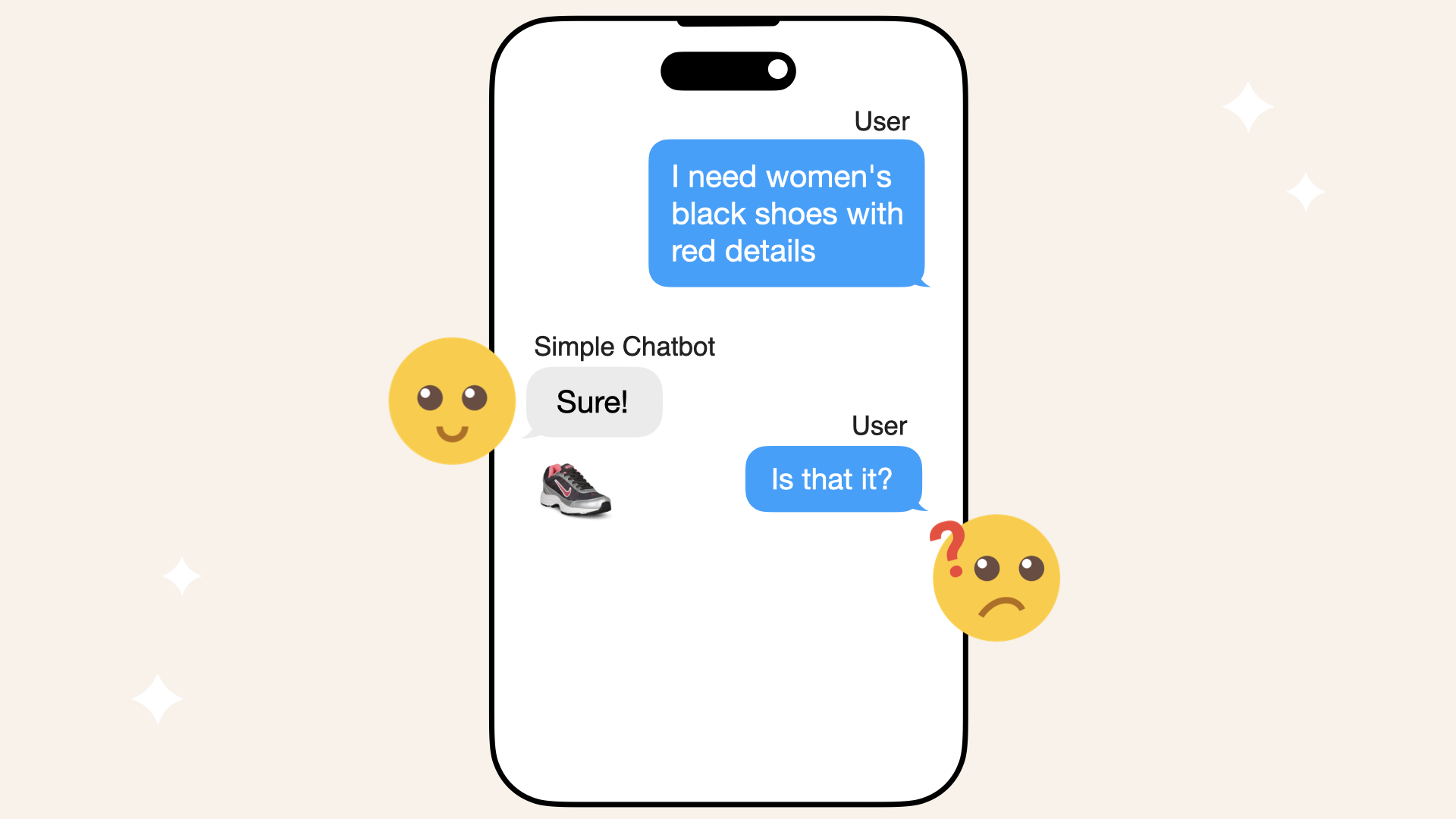
Customer: "I need women's black shoes with red details":

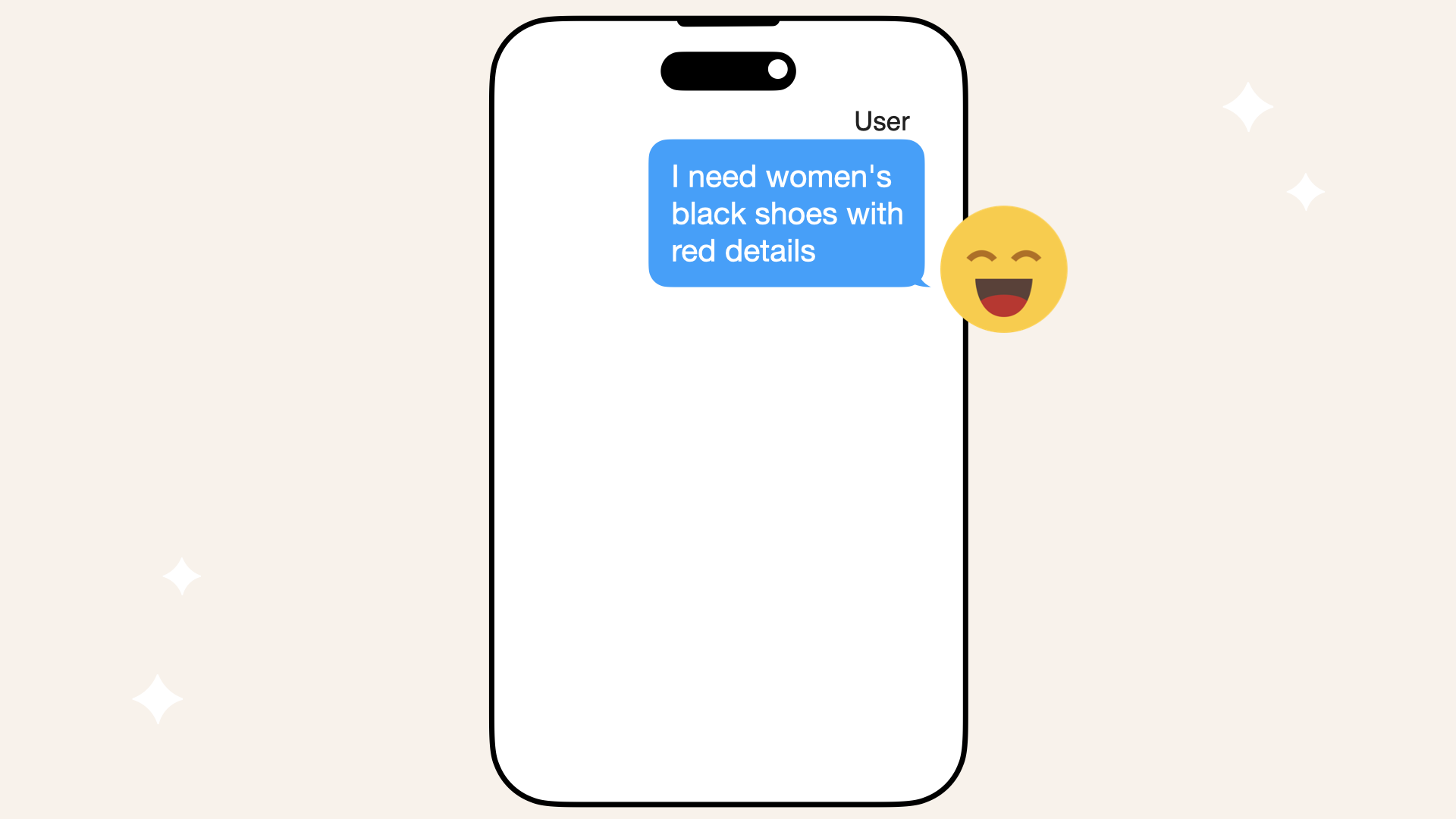
A customer initiates a chat with SoleMates

A customer initiates a chat with SoleMates and asks about women's black shoes with red details

Let's see how a naive chatbot handles this request.

Install dependencies

We'll use several libraries for this walkthrough, so let's start by installing all the dependencies.

note

The image folder with all the shoe images for SoleMates is 134.2 MB

Clone the GitHub repository to get started:

git clone https://github.com/norahsakal/solemates-data.git

Then navigate to the cloned folder:

cd solemates-data

Inside the folder, you'll find:

CSV file: data/solemates_shoe_directory.csv (product data)
For convenience, a pre-embedded dataset with all text and image embeddings is also available: data/solemates_shoe_directory_with_embeddings_token_count.csv
Image folder: footwear (shoe images, ~134 MB)

Next, pip install all the dependencies:

pip install -r requirements.txt

Then go ahead and launch Jupyter Notebook and create a new empty Jupyter Notebook:

jupyter notebook

Before we start to work with our shoe data, add all the necessary imports in the first cell of your Jupyter Notebook:

Jupyter Notebook
import ast
import base64
from datetime import datetime
import json
import os
from typing import Any, List, Optional

import boto3
from botocore.exceptions import NoCredentialsError
from IPython.display import display, Image, HTML

# LlamaIndex
from llama_index.core import Document
from llama_index.core import Settings
from llama_index.core import VectorStoreIndex

from llama_index.core.embeddings import BaseEmbedding
from llama_index.core.ingestion import IngestionPipeline
from llama_index.core.schema import QueryBundle
from llama_index.core.tools import FunctionTool

# LlamaIndex agents
from llama_index.core.agent import FunctionCallingAgentWorker, AgentRunner

# LlamaIndex LLMs
from llama_index.llms.openai import OpenAI as OpenAI_Llama

# LlamaIndex metadata filters
from llama_index.core.vector_stores.types import (
    MetadataFilters,FilterCondition
)

# LlamaIndex retrievers
from llama_index.core.retrievers import VectorIndexAutoRetriever, VectorIndexRetriever

# LlamaIndex vector stores
from llama_index.core.vector_stores import MetadataInfo, VectorStoreInfo
from llama_index.vector_stores.pinecone import PineconeVectorStore
from llama_index.core.vector_stores.types import VectorStoreQuery

# Pinecone
from pinecone import Pinecone, ServerlessSpec

import pandas as pd
from rapidfuzz import fuzz, process
from tqdm import tqdm
from tqdm.autonotebook import tqdm

Load shoe data

Let's start by reading the SoleMates shoe dataset.

We'll transform this data into embeddings and later store everything in the cloud-based Pinecone vector database.

Go ahead and load the dataset:

Jupyter Notebook
# Load the SoleMates shoe dataset
df_shoes = pd.read_csv('data/solemates_shoe_directory.csv')

# Convert 'color_details' from string representation of a list to an actual list
df_shoes['color_details'] = df_shoes['color_details'].apply(ast.literal_eval)

# Display the first few rows of the dataset
df_shoes.head()

You'll see this table in your Notebook:

http://localhost:3000/notebooks/jupyter_notebook.ipynb

product_title	gender	product_type	color	usage	color_details	heel_height	heel_type	price_usd	brand	product_id	image
Puma men future cat remix sf black casual shoes	men	casual shoes	black	casual	[]	nan	nan	220	puma	1	1.jpg
Buckaroo men flores black formal shoes	men	formal shoes	black	formal	[]	nan	nan	155	buckaroo	2	2.jpg
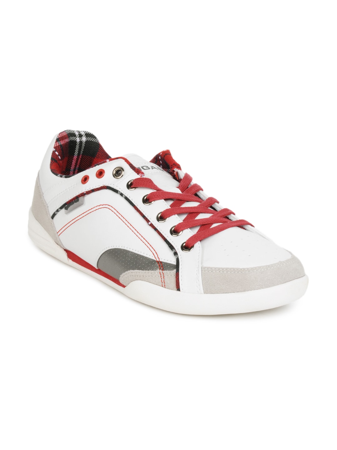
Gas men europa white shoes	men	casual shoes	white	casual	[]	nan	nan	105	gas	3	3.jpg
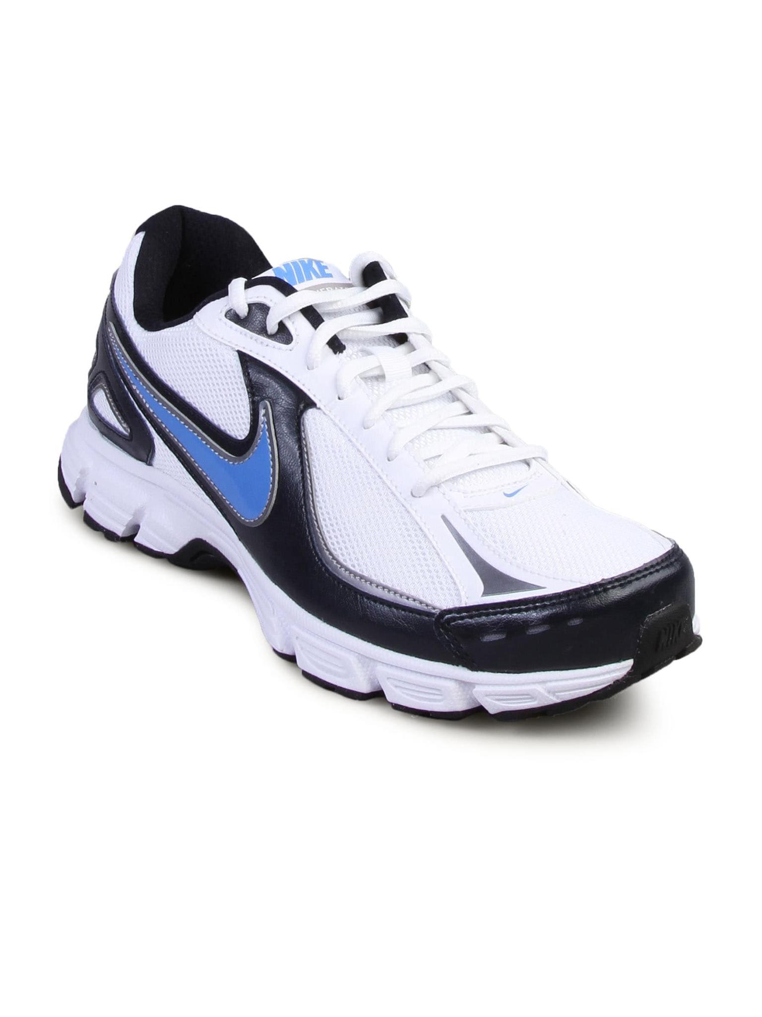
Nike men's incinerate msl white blue shoe	men	sports shoes	white	sports	['blue']	nan	nan	125	nike	4	4.jpg
Clarks men hang work leather black formal shoes	men	formal shoes	black	formal	[]	nan	nan	220	clarks	5	5.jpg

Let's also have a look at the first 5 shoes:

Jupyter Notebook
width = 100
images_html = ""
image_data_path = 'data/footwear'
for img_file in df_shoes.head()['image']:
    img_path = os.path.join(image_data_path, img_file)
    # Add each image as an HTML <img> tag
    images_html += f'<img src="{img_path}" style="width:{width}px; margin-right:10px;">'
# Display all images in a row using HTML
display(HTML(f'<div style="display: flex; align-items: center;">{images_html}</div>'))

Run this cell and it should look something like this:

Cost of vectorization

The next step is to vectorize the shoe product data:

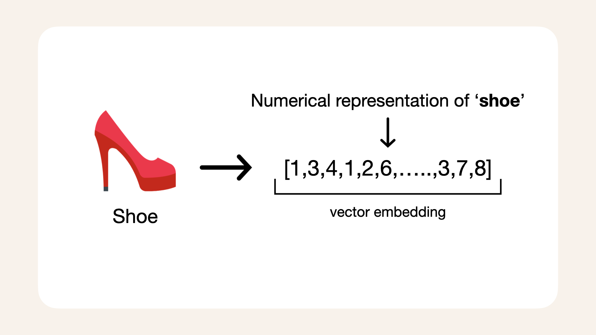
We need to generate a vector, the numerical representation of each shoe in our shoe database

Vectorizing datasets with AWS Bedrock and the Titan multimodal model involves costs based on the number of input tokens and images:

Text embeddings: $0.0008 per 1,000 input tokens
Image embeddings: $0.00006 per image

The provided SoleMates shoe dataset is fairly small, containing 1306 pair of shoes, making it affordable to vectorize.

For this dataset, I calculated the cost of vectorization and summarized the token counts below:

Token count: 12746 tokens
Images: 1306
Total cost: $0.0885568

Calculations:

(12746 tokens/1000)*0.0008 + (1306*0.00006) =
0.0885568

Pre-embedded dataset

Note

This step is entirely optional and designed to accommodate various levels of access and resources.

If you prefer not to generate embeddings or don't have access to AWS, you can use a pre-embedded dataset included in the repository.

This file contains all the embeddings and token counts, so you can follow this guide without incurring additional costs.

tip

For hands-on experience, I recommend running the embedding process yourself to understand the workflow better.

The pre-embedded dataset is located at:

data/solemates_shoe_directory_with_embeddings_token_count.csv

To load the dataset in your Jupyter Notebook, use the following code:

Jupyter Notebook
df_shoes_with_embeddings = pd.read_csv('data/solemates_shoe_directory_with_embeddings_token_count.csv')

# Convert string representations to actual lists
df_shoes_with_embeddings['titan_embedding'] = df_shoes_with_embeddings['titan_embedding'].apply(ast.literal_eval)

By using this pre-embedded dataset, you can skip the embedding step and continue directly with the rest of the walkthrough.

Note

This step is entirely optional and designed to accommodate various levels of access and resources.

For hands-on experience, I recommend running the embedding process to understand the workflow.

Prepare Amazon Bedrock for embedding generation

To vectorize our shoe product data, we'll generate embeddings for each product using AWS Titan multimodal model, so we need access to Amazon Bedrock models.

These embeddings combine image and text data to represent each shoe, allowing us to use semantic search on text, image or both image and text.

What is AWS Titan?

Amazon Titan Multimodal Embeddings G1 model is a multimodal embedding model that converts both product texts and images into vectors.

Learn more about AWS Titan G1 ↗

Why use AWS Titan?

A multimodal model allows us to process a query like "red heels" and match it to not only product descriptions but also actual images of red heels in the database.

By combining text and image data, the model helps the AI agent provide more relevant and visually aligned recommendations based on the customer's input.

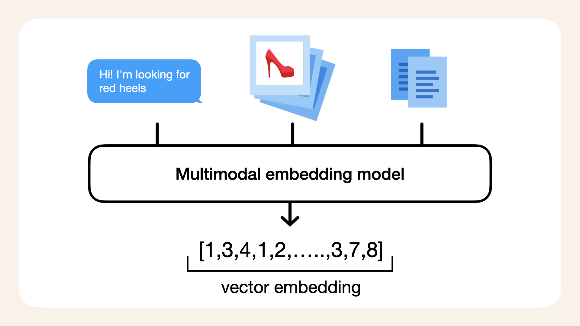
AWS Titan is a multimodal model, accepting images, text or both images and text

Getting started with Amazon Bedrock

To use Amazon Bedrock to generate embeddings for our shoes, start by setting up you AWS environment:

Create an AWS account if you don't already have one
Set up an AWS Identity and Access Management (IAM) roles with permissions tailored for Amazon Bedrock
Submit a request to access the foundational models (FMs) you'l like to use

In our case, we need access to the Titan Multimodal Embeddings G1 model.

Next, we'll initialize the Bedrock runtime client, which allows us to interact with AWS Titan to generate embeddings.

Set up AWS Bedrock client

Add this code snippet to a new Jupyter Notebook cell, leave aws_profile as None to use your default AWS profile:

Jupyter Notebook
# Define your AWS profile
# Replace AWS_PROFILE with the name of your AWS CLI profile
# To use your default AWS profile, leave 'aws_profile' as None
aws_profile = os.environ.get('AWS_PROFILE')

# Specify the AWS region where Bedrock is available
aws_region_name = "us-east-1"

try:
    # Set the default session for the specified profile
    if aws_profile:
        boto3.setup_default_session(profile_name=aws_profile)
    else:
        boto3.setup_default_session()  # Use default AWS profile if none is specified

    # Initialize the Bedrock runtime client
    bedrock_runtime = boto3.client(
        service_name="bedrock-runtime",
        region_name=aws_region_name
    )
except NoCredentialsError:
    print("AWS credentials not found. Please configure your AWS profile.")
except Exception as e:
    print(f"An unexpected error occurred: {e}")

Generate embeddings

Before we start to generate embeddings, we'll need to initialize two new columns in our dataset:

titan_embedding: to store the embedding vectors
token_count: to store the token count for each product title

Skip this step if using the pre-embedded dataset

Skip this step if you're using the pre-embedded dataset, since it already has these two columns

Jupyter Notebook
# Initialize columns to store embeddings and token counts
df_shoes['titan_embedding'] = None  # Placeholder for embedding vectors
df_shoes['token_count'] = None  # Placeholder for token counts

Next, let's define a function to generate embeddings and apply it to the dataset:

Jupyter Notebook
# Main function to generate image and text embeddings
def generate_embeddings(df, image_col='image', text_col='product_title', embedding_col='embedding', image_folder=None):

    if image_folder is None:
        raise ValueError("You must specify an image folder path.")

    for index, row in tqdm(df.iterrows(), total=df.shape[0], desc="Generating embeddings"):
        try:
            # Prepare image file as base64
            image_path = os.path.join(image_folder, row[image_col])
            with open(image_path, 'rb') as img_file:
                image_base64 = base64.b64encode(img_file.read()).decode('utf-8')

            # Create input data for the model
            input_data = {"inputImage": image_base64, "inputText": row[text_col]}

            # Invoke AWS Titan model via Bedrock runtime
            response = bedrock_runtime.invoke_model(
                body=json.dumps(input_data),
                modelId="amazon.titan-embed-image-v1",
                accept="application/json",
                contentType="application/json"
            )
            response_body = json.loads(response.get("body").read())

            # Extract embedding and token count from response
            embedding = response_body.get("embedding")
            token_count = response_body.get("inputTextTokenCount")

            # Validate and save the embedding
            if isinstance(embedding, list):
                df.at[index, embedding_col] = embedding  # Save embedding as a list
                df.at[index, 'token_count'] = int(token_count)  # Save token count as an integer
            else:
                raise ValueError("Embedding is not a list as expected.")

        except Exception as e:
            print(f"Error for row {index}: {e}")
            df.at[index, embedding_col] = None  # Handle errors gracefully

    return df

When you've added this function, run this next cell to start generating embeddings:

This next function will start generating vectors and inquire a cost

Running this next function will start calling Amazon Bedrock and inquire a total cost of $0.09.

This whole process takes around 10 minutes.

Jupyter Notebook
# Generate embeddings for the product data
df_shoes = generate_embeddings(df=df_shoes, embedding_col='titan_embedding')

This will start a progress bar where you'll see the process. It takes approximately 10 minutes to generate embeddings for the 1306 pair of shoes in our shoe database.

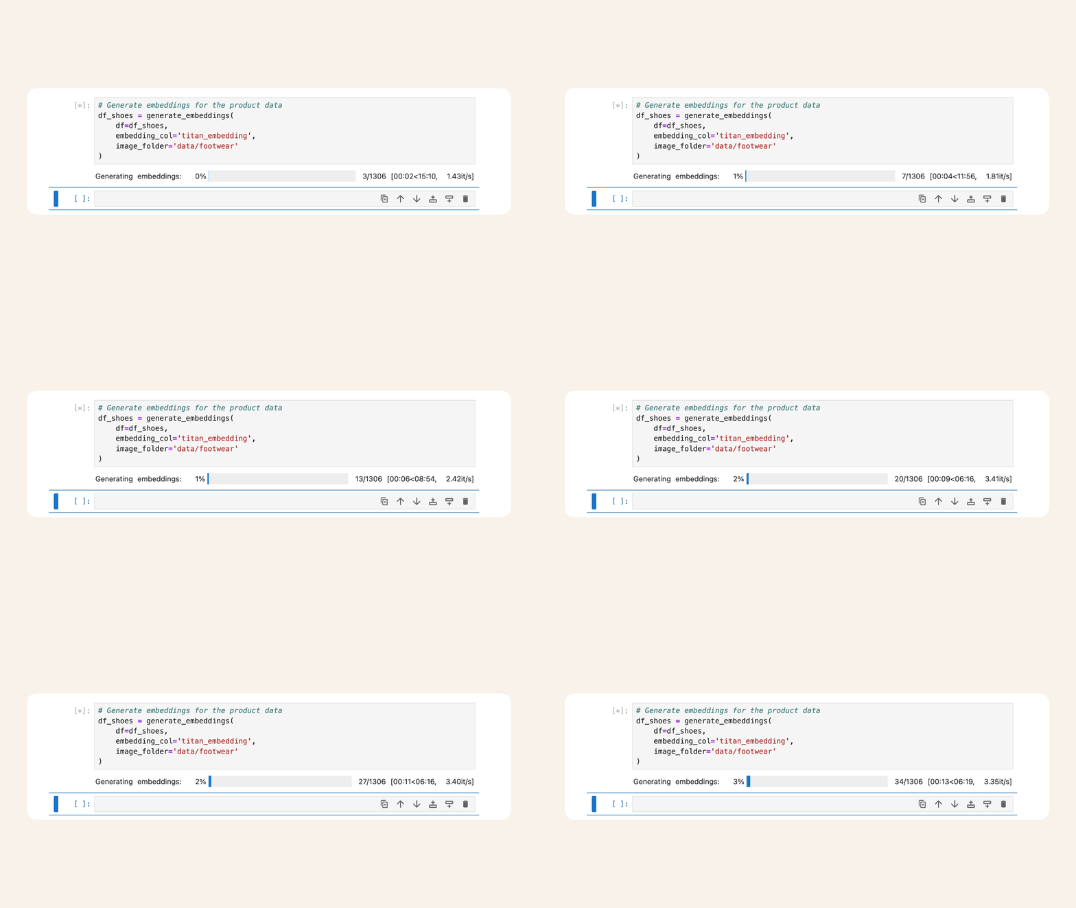
The vectorization of 1306 shoes takes approximately 10 minutes

Once all shoes are processed, make sure to save the dataset for reuse, so you don't have to generate new embeddings for this dataset:

Jupyter Notebook
# Save the dataset with generated embeddings to a new CSV file
# Get today's date in YYYY_MM_DD format
today = datetime.now().strftime('%Y_%m_%d')

# Save the dataset with generated embeddings to a CSV file
df_shoes.to_csv(f'shoes_with_embeddings_token_{today}.csv', index=False)
print(f"Dataset with embeddings saved as 'shoes_with_embeddings_token_{today}.csv'")

Create a dictionary with product data

The next step is to create LlamaIndex Document object, but first we need to structure the product data into dictionaries.

These dictionaries include:

Text: The product title that will be used for embedding queries
Metadata: A dictionary containing detailed attributes for each shoe (e.g., color, gender, usage, price)
Embedding: The AWS Titan embeddings generated earlier

We're creating this dictionary format to structure our data before creating the LlamaIndex Document object in the next step:

Jupyter Notebook
# Convert DataFrame rows into a list of dictionaries for LlamaIndex
product_data = df_shoes.apply(lambda row: {
    'text': row['product_title'],
    'metadata': {
        'color': row['color'],
        'text': row['product_title'],
        'gender': row['gender'],
        'product_type': row['product_type'],
        'usage': row['usage'],
        'price': row['price_usd'],
        'product_id': row['product_id'],
        'brand': row['brand'],
        **({'heel_height': float(row['heel_height'])} if not pd.isna(row['heel_height']) else {}),
        **({'heel_type': row['heel_type']} if not pd.isna(row['heel_type']) else {}),
        **({'color_details': row['color_details']} if row['color_details'] else {})
    },
    'embedding': row['titan_embedding']
}, axis=1).tolist()

# Preview the first product dictionary
#product_data[0]

Create LlamaIndex Documents

We'll now use the product data dictionaries to create LlamaIndex Document objects.

Why create LlamaIndex Documents?

These Documents are crucial because:

They act as containers for our product data and embeddings
They enable seamless interaction with Pinecone for upserting embeddings

Learn more about LlamaIndex Documents ↗

Each LlamaIndex Document includes:

The text (shoe product title) for embedding and query purposes
Metadata with attributes like color, gender, price etc.
The embedding we generated earlier
An exclusion list (excluded_embed_metadata_keys) to prevent unnecessary fields from being embedded by LlamaIndex

Run this next snippet in your Jupyter Notebook to create the LlamaIndex Documents:

Jupyter Notebook
# Create LlamaIndex Document objects
documents = []
for doc in product_data:
    documents.append(
        Document(
            text=doc["text"],
            extra_info=doc["metadata"],
            embedding=doc['embedding'],

            # Avoid embedding unnecessary metadata
            excluded_embed_metadata_keys=[
                'color',
                'gender',
                'product_type',
                'usage',
                'text',
                'price',
                'product_id',
                'brand',
                'heel_height',
                'heel_type',
                'color_details'
            ]
        )
    )

# Confirm the first Document object
documents[0].metadata

The first shoe metadata should be the following:

{'color': 'black',
 'text': 'Puma men future cat remix sf black casual shoes',
 'gender': 'men',
 'product_type': 'casual shoes',
 'usage': 'casual',
 'price': 220,
 'product_id': 1,
 'brand': 'puma'}

Initialize Pinecone

Alright, we have the vectors and prepared the Documents so we're ready to upsert our vectors and data to cloud-based Pinecone vector database.

To interact with Pinecone, you'll first need an account and API keys.

If you don't already have them, create a Pinecone account and retrieve your API key.

What is Pinecone?

Pinecone is a vector database which you can use for text similarity search tasks, such as sentiment analysis, text classification and question answering.

Learn more about Pinecone ↗

We'll use Pinecone to upsert the AWS Titan G1 embeddings we generated earlier, enabling both similarity and hybrid search.

Start by initializing the Pinecone client with your API key:

Jupyter Notebook
# Initialize Pinecone client with API key
pc = Pinecone(api_key=os.environ['PINECONE_API_KEY'])
index_name = "solemates"  # Replace with your desired index name

List current indexes

Let's list the existing indexes in your Pinecone account to ensure no duplicates before we create a new index:

Jupyter Notebook
# List current indexes
pc.list_indexes()

You should see this cell output:

{'indexes': []}

Create new index

Next, we'll create a new Pinecone index. An index stores the embeddings and metadata for our shoe data.

Dimension: Matches the size of the embeddings we're using (1024 for AWS Titan G1 multimodal embeddings)
Metric: Defines how similarity is calculated (e.g., dot product, cosine similarity)
ServerlessSpec: Specifies the cloud provider and region for your index

Run this next snippet, if the index already exists, this step will be skipped:

Jupyter Notebook
if index_name not in pc.list_indexes().names():
    pc.create_index(
        name=index_name, # The index name you picked earlier
        dimension=1024,  # AWS Titan embeddings require 1024 dimensions
        metric="dotproduct",  # Required for hybrid search with Pinecone
        spec=ServerlessSpec(
            cloud="aws",
            region="us-east-1"
        )
    )

Why dot product instead of cosine similarity?

Cosine similarity is a popular metric for semantic search but in our case want to be able to do hybrid search and as of January 20, 2025, Pinecone requires dot product as metric for hybrid search.

Learn more about hybrid search in Pinecone ↗

If you run this cell again:

Jupyter Notebook
# List current indexes
pc.list_indexes()

You'll see the newly created index as a cell output:

http://localhost:3000/notebooks/jupyter_notebook.ipynb

{'indexes': [{'deletion_protection': 'disabled',
              'dimension': 1024,
              'host': 'solemates-xxxxxxx.svc.aped-xxxx-xxxx.pinecone.io',
              'metric': 'dotproduct',
              'name': 'solemates',
              'spec': {'serverless': {'cloud': 'aws', 'region': 'us-east-1'}},
              'status': {'ready': True, 'state': 'Ready'}}]}

Inspect Pinecone

Navigate to you Pinecone dashboard, and you should now see your new index with 0 records (vectors), as it hasn't been populated with our vectors yet:

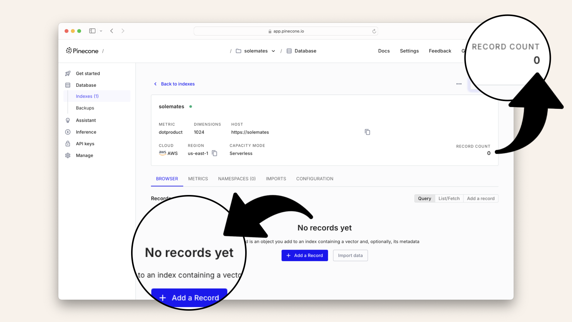
Your newly created Pinecone index is currently empty

Initialize Pinecone index

After creating the index, we'll initialize it to be able to upsert our embeddings and later query the vectors:

Jupyter Notebook
pinecone_index = pc.Index(index_name)

Create Pinecone vector store

We'll now ser up a Pinecone Vector Store using LlamaIndex.

The vector store connects our Pinecone index with the LlamaIndex framework.

Key configuration details:

Namespace: A logical grouping within the index, allowing future addition of other product types
Hybrid search: Enabling both semantic and keyword search by adding sparse vectors in addition to dense vectors

tip

Learn more about namespaces and hybrid search:

Go ahead and create the Pinecone vector store in your Jupyter Notebook:

Jupyter Notebook
vector_store = PineconeVectorStore(
    pinecone_index=pinecone_index,
    namespace='footwear',  # Logical namespace for shoe data
    add_sparse_vector=True  # Enables hybrid search
)

Create an ingestion pipeline

We'll create an IngestionPipeline with LlamaIndex to upsert our vectors into the Pinecone index we created. No transformations are required since we've pre-generated our embeddings with AWS Titan.

note

As of January 20 2025, LlamaIndex doesn't abstract AWS Titan G1 multimodal embeddings, so we're using our own vectors directly.

Define your IngestionPipeline in your Jupyter Notebook:

Jupyter Notebook
pipeline = IngestionPipeline(
    transformations=[],  # No transformations since we pre-generated our embeddings
    vector_store=vector_store
)

Run the ingestion pipeline

This step upserts the embeddings into Pinecone for storage and querying.

Cost note

Pinecone charges $2 per 1 million vectors unless you're on the free plan
It may take a minute or two for the vectors to become visible in your Pinecone index

Run the IngestionPipeline to start upserting our vectors into Pinecone, this might take a minute or so:

Jupyter Notebook
# Run the pipeline to upsert embeddings into Pinecone
pipeline.run(documents=documents, show_progress=True)

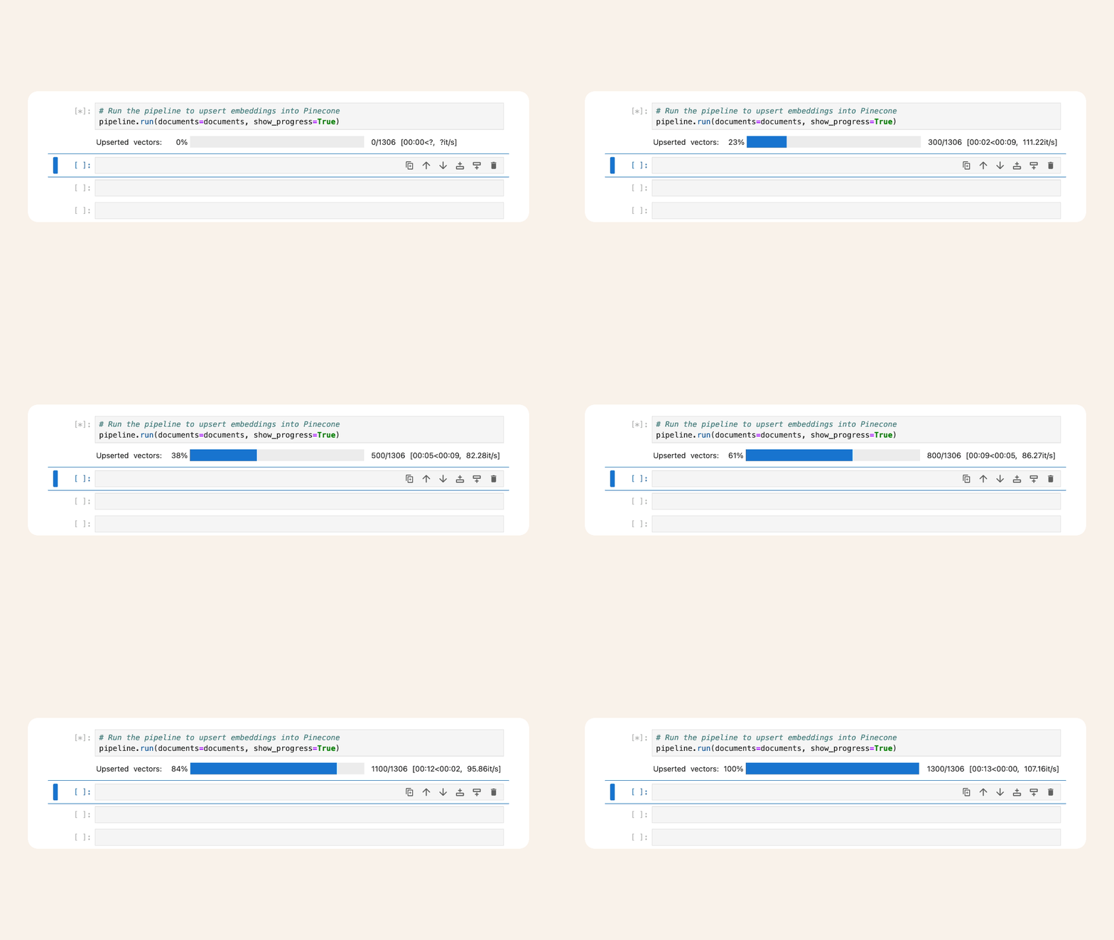
The IngestionPipeline upserts our vectors, which might take a minute or so

Inspect your Pinecone index

Now that we've upserted the vectors, navigate back to you Pinecone dashboard. You should now see 1306 records in your index, corresponding to the 1306 shoes we vectorized and upserted:

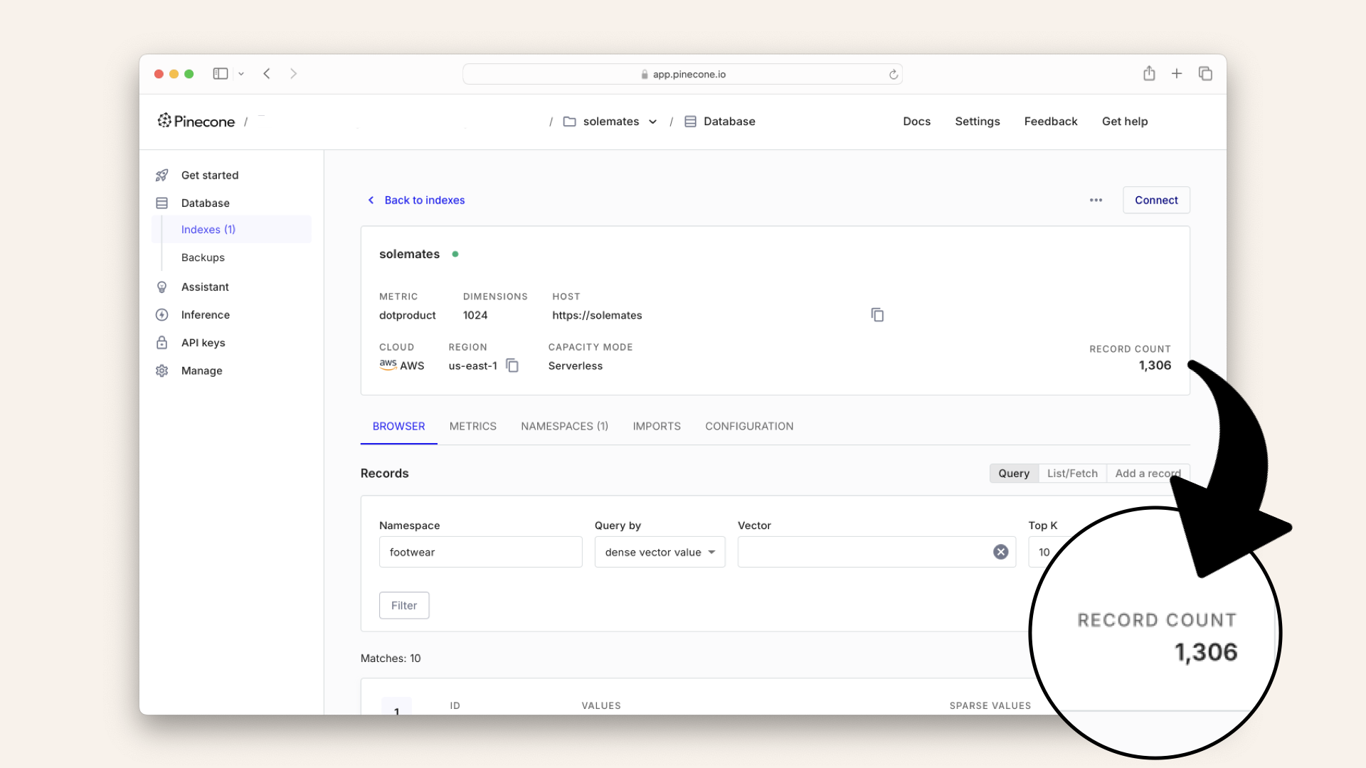
You should now see 1306 records in your index

Test querying the vector store

Now that we have upserted all our shoe vectors, let's test querying the vector database.

We'll do that by creating a Vector Store Index with LlamaIndex. This index will allow us to query the Pinecone index using the same vector store we initialized earlier.

Create a vector store index in your Jupyter Notebook:

Jupyter Notebook
# Create a Vector Store Index
vector_index = VectorStoreIndex.from_vector_store(vector_store=vector_store)

Query the vector database directly

Before we use a Query Engine or Chat Engine to interact with the vector database, let's start with a direct query using a simple LlamaIndex retriever.

Why use a simple retriever?

This approach demonstrates how you can fetch relevant records from the vector database without involving advanced reasoning, natural language understanding, or conversation tracking.

It's a fundamental way to confirm that the embeddings and metadata are stored correctly and that the vector database is functioning as expected.

Advanced querying techniques later on

We'll move on to more advanced querying techniques, including using a Query engine and an Agent to leverage the power of LLMs later in this guide.

The first step is creating a simple retriever, but first, we need to define a custom embedding function.

Why we need a custom embedding class

As of January 20, 2025, LlamaIndex does not abstract AWS Titan multimodal embeddings, so we'll implement a custom class for this purpose

Create a function to request AWS Titan embeddings

We'll define a helper function to request AWS Titan multimodal embeddings.

This function will handle both text and image inputs:

Jupyter Notebook
def request_embedding(image_base64=None, text_description=None):
    """
    Request embeddings from AWS Titan multimodal model.

    Parameters:
        image_base64 (str, optional): Base64 encoded image string.
        text_description (str, optional): Text description.

    Returns:
        list: Embedding vector.
    """
    input_data = {"inputImage": image_base64, "inputText": text_description}
    body = json.dumps(input_data)

    # Invoke the Titan multimodal model
    response = bedrock_runtime.invoke_model(
        body=body,
        modelId="amazon.titan-embed-image-v1",
        accept="application/json",
        contentType="application/json"
    )

    response_body = json.loads(response.get("body").read())

    if response_body.get("message"):
        raise ValueError(f"Embeddings generation error: {response_body.get('message')}")

    return response_body.get("embedding")

Create custom embedding class

We'll now define a custom embedding class that uses the AWS Titan multimodal model to generate embeddings via the function we just defined.

This class overrides key methods in LlamaIndex's BaseEmbedding to integrate AWS Titan into the framework.

Define the custom embedding class in your Jupyter Notebook:

Jupyter Notebook
class MultimodalEmbeddings(BaseEmbedding):
    """
    Custom embedding class for AWS Titan multimodal embeddings.
    """

    def __init__(self, **kwargs: Any) -> None:
        super().__init__(**kwargs)

    @classmethod
    def class_name(cls) -> str:
        return "multimodal"

    async def _aget_query_embedding(self, query: str) -> List[float]:
        return self._get_query_embedding(query)

    async def _aget_text_embedding(self, text: str) -> List[float]:
        return self._get_text_embedding(text)

    def _get_query_embedding(self, query: str) -> List[float]:
        """
        Get embeddings for a query string.
        """
        return request_embedding(text_description=query)

    def _get_text_embedding(self, text: str) -> List[float]:
        """
        Get embeddings for a text string.
        """
        return request_embedding(text_description=text)

    def _get_text_embeddings(self, texts: List[str]) -> List[List[float]]:
        """
        Get embeddings for a batch of text strings.
        """
        return [request_embedding(text_description=text) for text in texts]

Instantiate the custom class

We'll now instantiate the MultimodalEmbeddings class we just defined to use it in our retriever:

Jupyter Notebook
# Instantiate the custom embedding model
embed_model = MultimodalEmbeddings()

Create a simple retriever

Let's create a simple retriever using the custom embedding model and our vector index.

Key configurations:

similarity_top_k: Number of top results to retrieve (neighbors in our vector database)
vector_store_query_mode: Set to "hybrid" for combining semantic and keyword search
alpha: Weighting between semantic (dense vectors) and keyword search (sparse vectors)

Create retriever

Add the retriever to your Jupyter Notebook:

Jupyter Notebook
# Create a simple retriever
retriever = VectorIndexRetriever(
    index=vector_index,
    embed_model=embed_model,
    similarity_top_k=8,  # Retrieve the top 8 results
    vector_store_query_mode="hybrid",  # Enable hybrid search
    alpha=0.5  # Weighting between semantic and keyword search
)

Why query the vector database directly with a simple retriever?

We're using this simple and straightforward retriever to query our vector database and inspect the results.

This method interacts with the embeddings and metadata in a straightforward way, without utilizing an LLM-powered Query Engine or Chat Engine.

Why this step matters

Validates that the vector database is populated correctly
Shows how to query embedding directly, bypassing the overhead of LLM-based reasoning
Prepares the groundwork for building advanced workflows with Query Engines and AI Agents

Query the vector store

Go ahead and query the Pinecone vector store with the input query "red shoes":

Jupyter Notebook
# Query the vector store for "red shoes"
results = retriever.retrieve("red shoes")

# Display results
for item in results:
    score = item.score
    print(f"Score: {score:.4f}")
    print(f"Text: {item.get_content()}")
    print("-" * 50)

You should see this output in you Jupyter Notebook:

http://localhost:3000/notebooks/jupyter_notebook.ipynb

Score: 2.2923
Text: Id men red shoes
--------------------------------------------------
Score: 2.2458
Text: Arrow men red shoes
--------------------------------------------------
Score: 2.2390
Text: Catwalk women red shoes
--------------------------------------------------
Score: 2.2381
Text: Vans men red old skool shoes
--------------------------------------------------
Score: 2.2366
Text: Cobblerz women red shoes
--------------------------------------------------
Score: 2.2335
Text: Converse men black & red shoes
--------------------------------------------------
Score: 2.2253
Text: Converse men red casual shoes
--------------------------------------------------
Score: 2.2251
Text: Fila men leonard red shoes
--------------------------------------------------

As seen, all shoes seem to be red.

Function to visualize the vector database pull

The vector database query returns a list of red shoes based on the embeddings. The verify the results, let's also look at the image of the actual shoes we pulled from the vector database.

Let's create a function that loops through the retrieved nodes and displays each image along with its metadata in a row for easy inspection:

Jupyter Notebook
def display_nodes_with_images_in_row(vector_database_response_nodes, image_folder_path=None, img_width=100):
    html_content = "<div style='display: flex; flex-wrap: wrap; gap: 20px;'>"

    if image_folder_path is None:
        raise ValueError("You must specify an image folder path.")

    for node in vector_database_response_nodes:
        # Retrieve text and product_id from node metadata
        text = node.metadata.get('text')
        product_id = node.metadata.get('product_id')

        # Generate image path based on product_id
        image_path = os.path.join(image_folder_path, f"{product_id}.jpg")

        if os.path.exists(image_path):
            # Add each text and image in a flex container
            html_content += f"""
                <div style="text-align: center;">
                    <p>{text}</p>
                    <img src='{image_path}' width='{img_width}px' style="padding: 5px;"/>
                </div>
            """
        else:
            # Handle missing images gracefully
            html_content += f"""
                <div style="text-align: center;">
                    <p>{text}</p>
                    <p style='color: red;'>Image not found for product_id {product_id}</p>
                </div>
            """

    # Close the main div
    html_content += "</div>"

    # Display the content as HTML
    display(HTML(html_content))

Visualize shoes

Now, let's call the function and visualize the shoes retrieved from the vector database to confirm that the results match the query "red shoes".

Run this snippet in your Jupyter Notebook:

Jupyter Notebook
display_nodes_with_images_in_row(results, image_folder_path='data/footwear')

You should now see these 8 shoes in the cell output in your Jupyter Notebook:

http://localhost:3000/notebooks/jupyter_notebook.ipynb

Id men red shoes

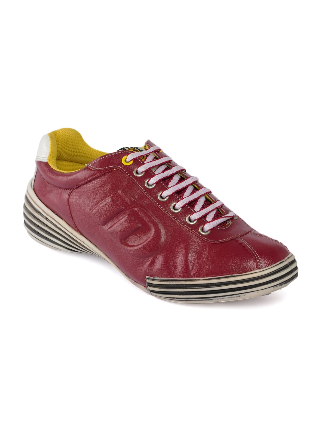
Arrow men red shoes

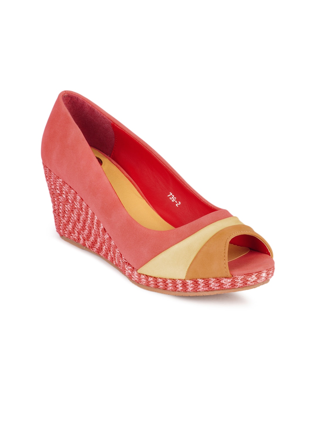
Catwalk women red shoes

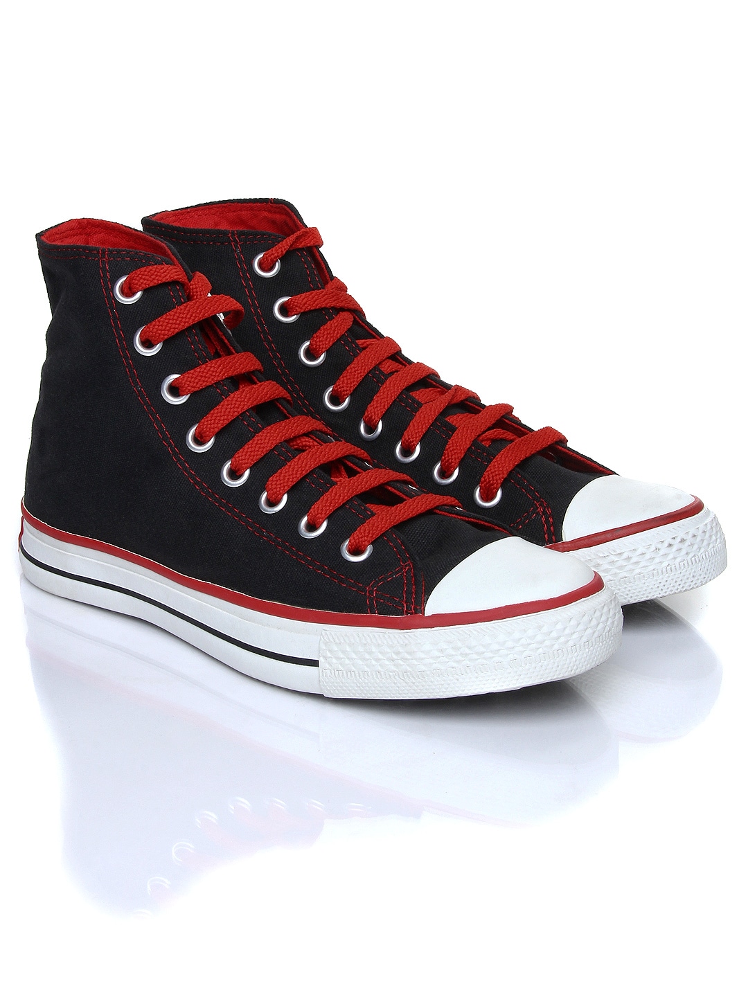
Vans men red old skool shoes

Cobblerz women red shoes

Converse men black & red shoes

Converse men red casual shoes

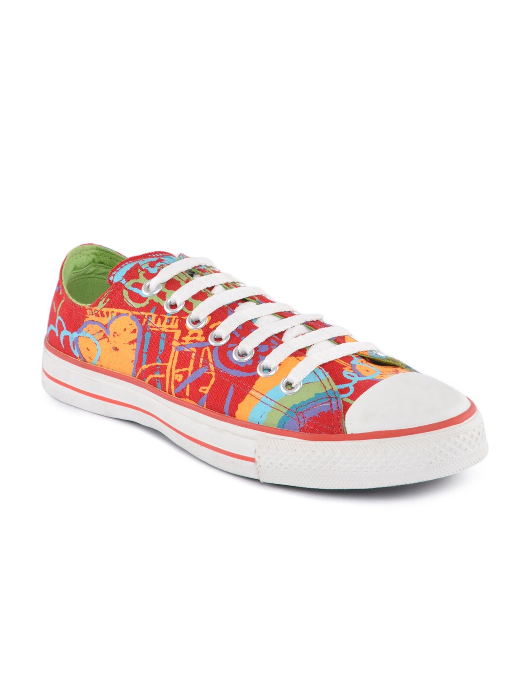
Fila men leonard red shoes

Examine the shoes

As shown, all the retrieved shoes are red or have red details, confirming that the naive vector index query works well for focused queries like red shoes:

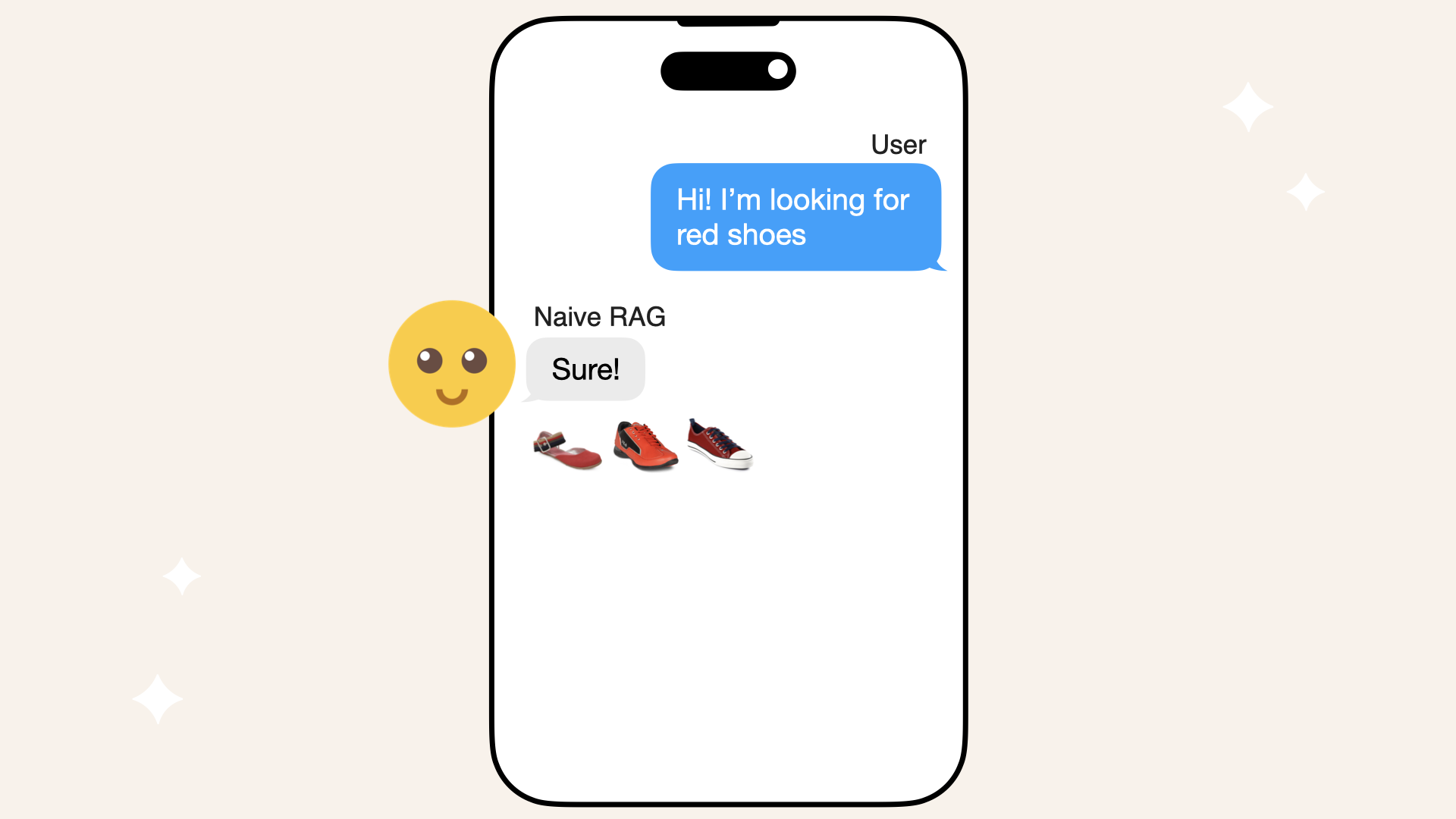
Focused queries like "red shoes" works well

Focused queries like "red shoes" works well, even without an LLM

Next, we'll involve an LLM to add more flexibility to our queries.

Why not keep using the index alone?

But the vector database pull of red shoes looks great, so why even involve an LLM?

Before we add an LLM, let's try to query the vector database again, but this time with something unrelated, like a "Thank you!" from the customer and examine the new response:

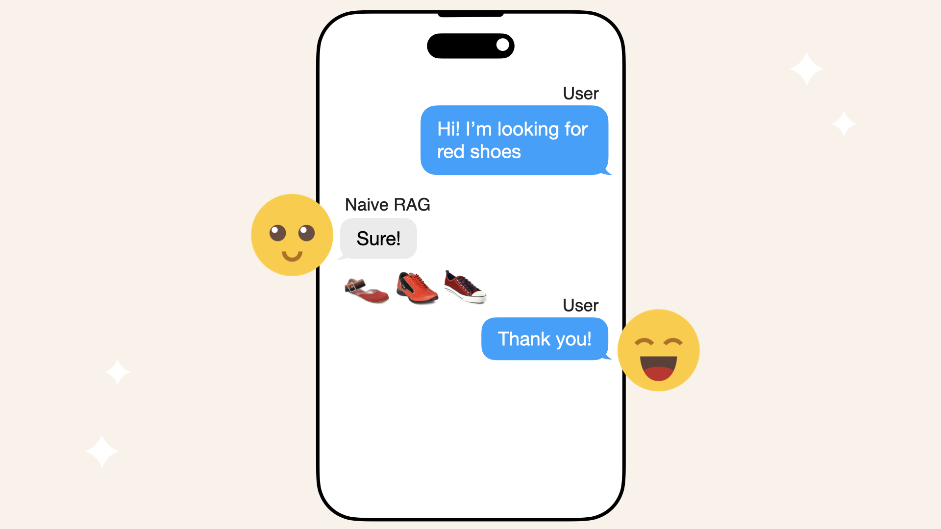
Try to query vector database with something unrelated, like "Thank you!"

Let's try to query our vector database with something unrelated, like "Thank you!"

Test the naive query

Run the snippet again, but this time, use the query "Thank you!":

Jupyter Notebook
# Query the vector store with an unrelated query
results = retriever.retrieve("Thank you!") # Try an unrelated query

# Display results
for item in results:
    score = item.score
    print(f"Score: {score:.4f}")
    print(f"Text: {item.get_content()}")
    print("-" * 50)

# Visualize the results
display_nodes_with_images_in_row(results)

You'll see this output from your Jupyter Notebook cell:

http://localhost:3000/notebooks/jupyter_notebook.ipynb

Score: 1.1846
Text: Timberland women femmes brown boot
--------------------------------------------------
Score: 1.1839
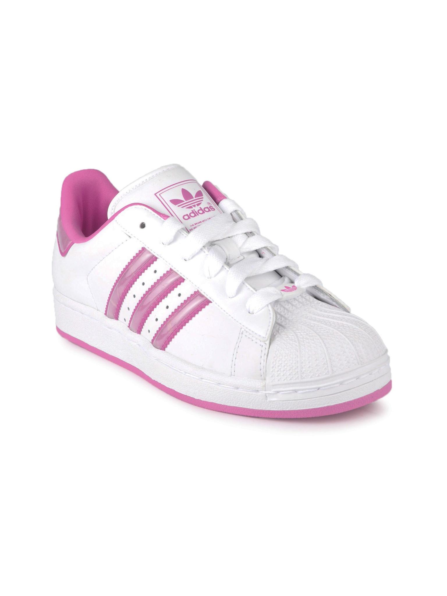
Text: Adidas women color can pink shoes
--------------------------------------------------
Score: 1.1784
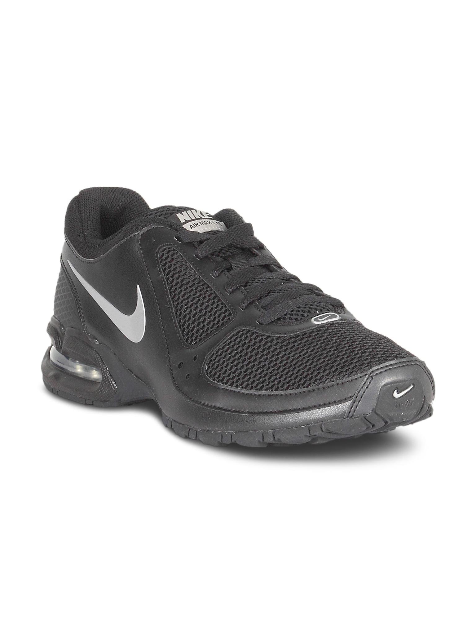
Text: Nike men's air max black shoe
--------------------------------------------------
Score: 1.1750
Text: Id men red shoes
--------------------------------------------------
Score: 1.1746
Text: Adidas originals women superstar 2 white casual shoes
--------------------------------------------------
Score: 1.1744
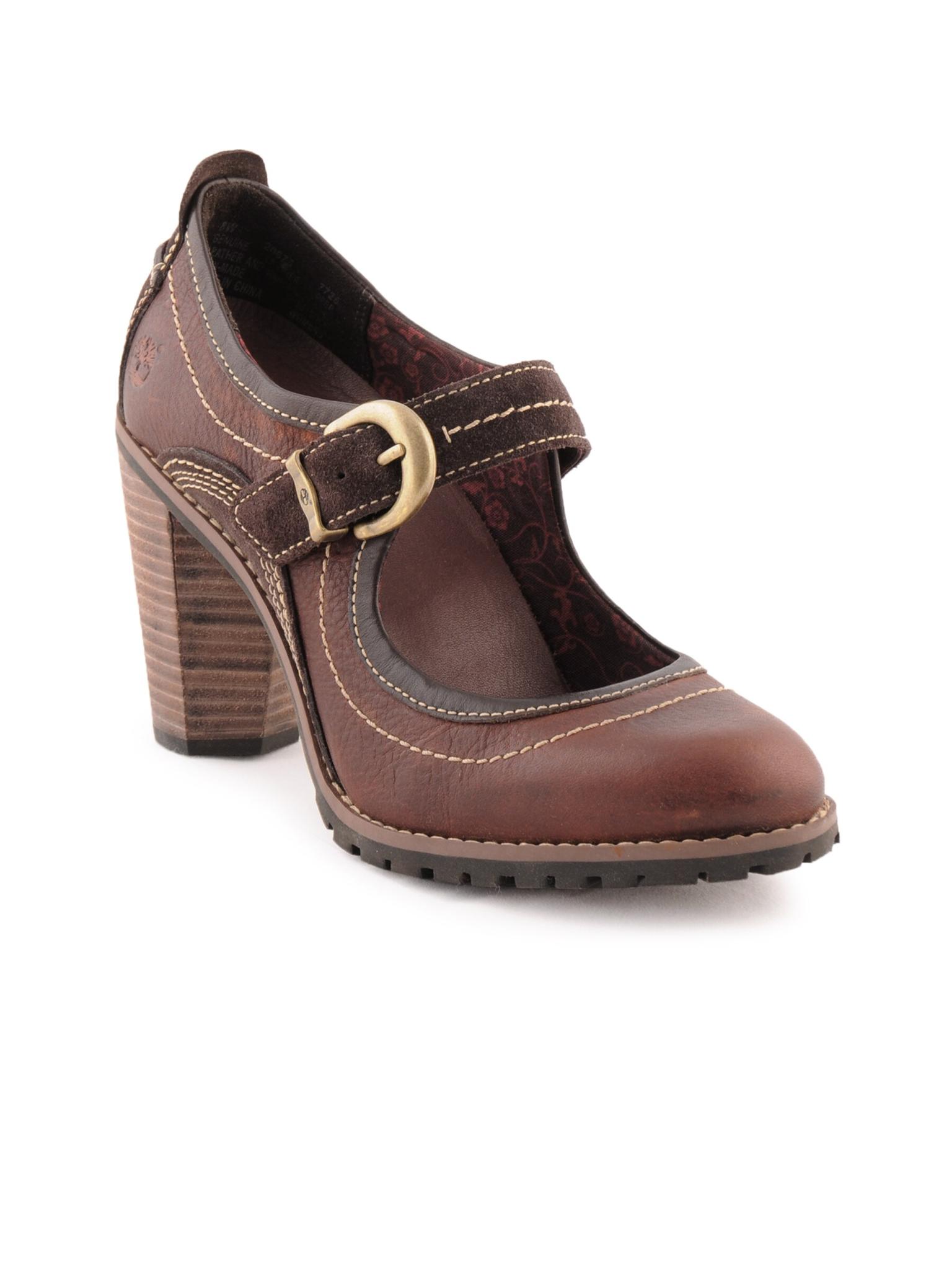
Text: Timberland women femmes brown casual shoes
--------------------------------------------------
Score: 1.1732
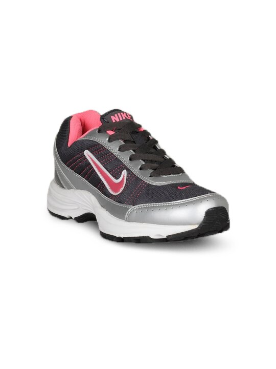
Text: Nike women's transform iii in black pink shoe
--------------------------------------------------
Score: 1.1726
Text: Vans men khaki shoes
--------------------------------------------------

And you'll see these shoes:

http://localhost:3000/notebooks/jupyter_notebook.ipynb

Timberland women femmes brown boot

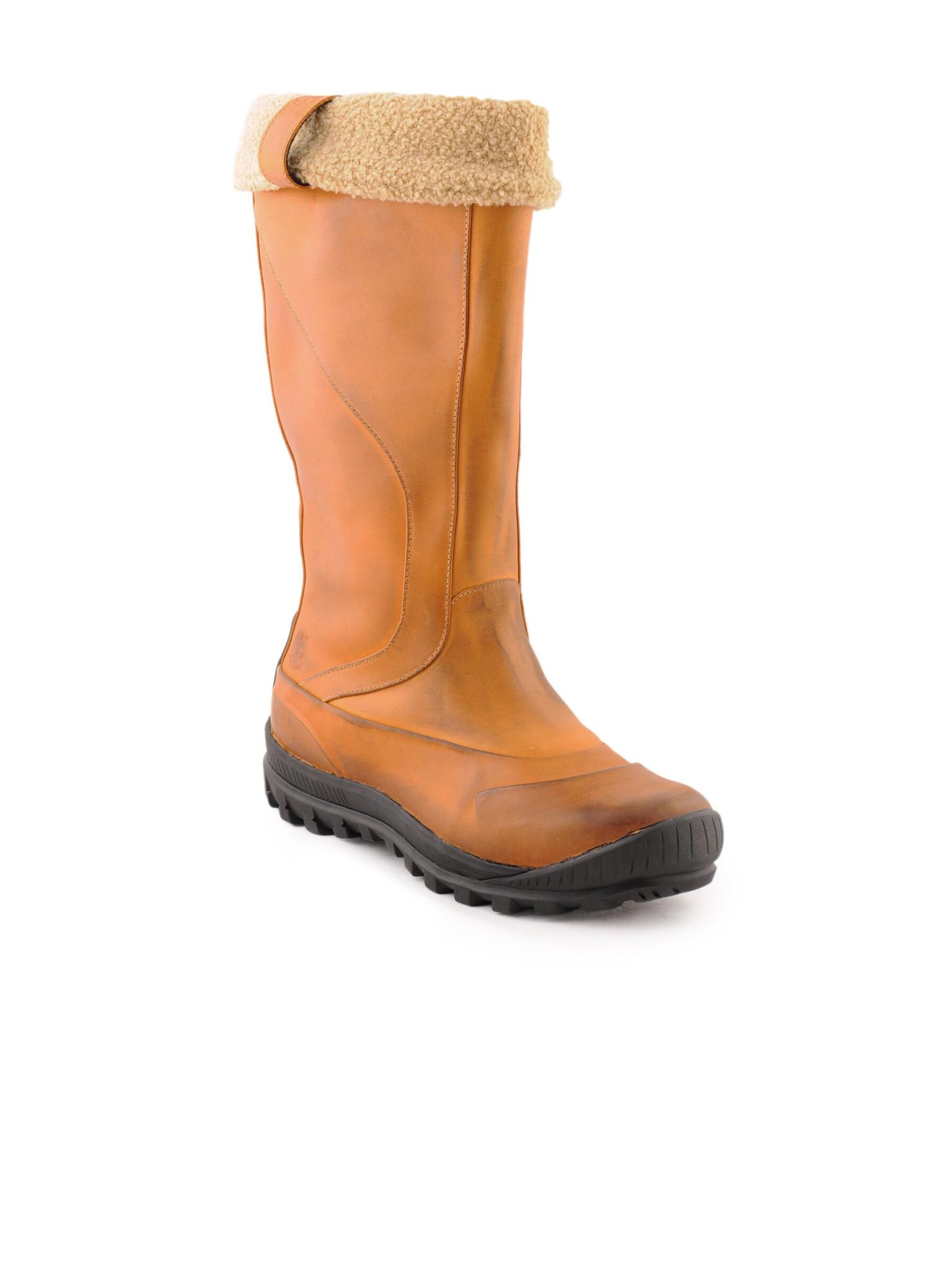
Adidas women color can pink shoes

Nike men's air max black shoe

Id men red shoes

Adidas originals women superstar 2 white casual shoes

Timberland women femmes brown casual shoes

Nike women's transform iii in black pink shoe

Vans men khaki shoes

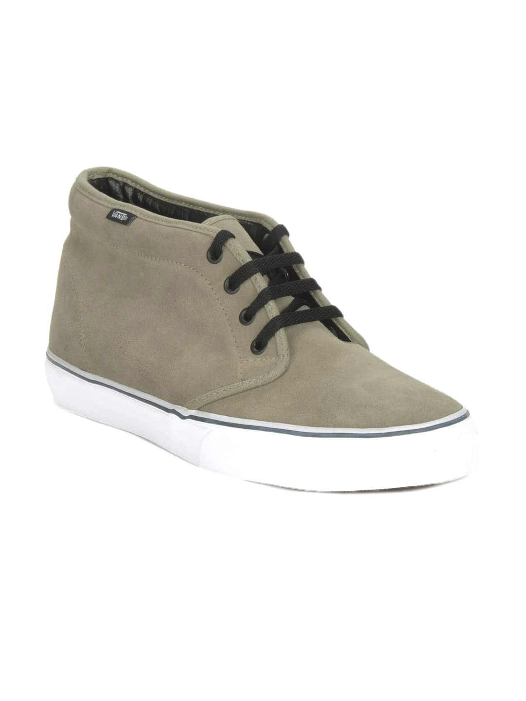
Limitations of a naive RAG system

As seen, regardless of the query, the vector database matches the closest vectors based on the embeddings.

In this case, querying with "Thank you!" still returns shoes that have vectors most similar to the vectorized "Thank you!":

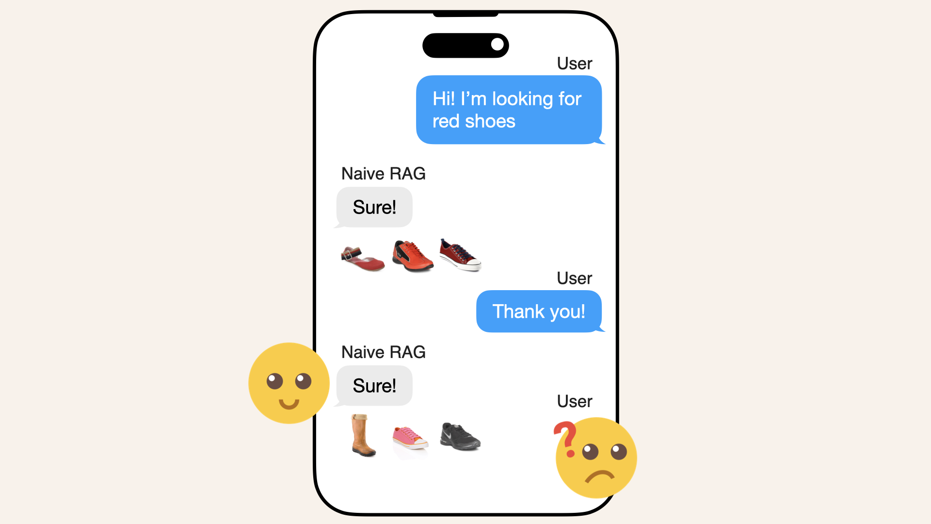
Querying with "Thank you!" still returns shoes that have vectors most similar to that query

Querying our vector database with "Thank you!" still returns shoes that have vectors most similar to that query

The naive RAG system doesn't understand the context or intent of the query and always replies with similar vectors.

This demonstrates the limitations of a naive RAG (Retrieval-Augmented Generation) system.

While this works well for focused queries like "red shoes", it fails to adapt to non-specific or conversational inputs.

Overcome naive RAG limitations: create a vector index query engine

To overcome the limitations of naive queries, we'll integrate an LLM into our workflow by creating a Query Engine.

This Query Engine will:

Interpret the user's natural language input
Retrieve contextually relevant products from the vector database
Enable more dynamic and flexible interactions with the data

For this guide, we'll use the openai-o4 model for the LLM.

Initialize LLM

Start by initializing the LLM in your Jupyter Notebook:

Jupyter Notebook
# Initialize LLM
llm = OpenAI_Llama(
    temperature=0.0,
    model="gpt-4o",
    api_key=os.environ["OPENAI_API_KEY"]
)
Settings.llm = llm

Create query engine

We'll now create a query engine using the vector index and our custom embedding model. This engine will leverage the LLM for a more intelligent query interpretation and responses.

Define the query engine in your Jupyter Notebook:

Jupyter Notebook
# Create a query engine from the vector index
query_engine = vector_index.as_query_engine(
    embed_model=embed_model,
    similarity_top_k=8,
    vector_store_query_mode="hybrid",
    alpha=0.5,
)

What is the alpha argument?

The alpha is a number weighting between full semantic similarity (dense embeddings) or full keyword search.

Test query engine with today's challenge: black shoes with red details

Let's test the query engine by asking for black shoes with red details:

Jupyter Notebook
# Query the engine for black-tie event shoes
response = query_engine.query("I need women's black shoes with red details")

print("Chatbot response: ", response.response)

The chatbot response is not deterministic so your reply might not be exactly the following, but here's the LLM response I received:

http://localhost:3000/notebooks/jupyter_notebook.ipynb

Chatbot response: The Nike women's transform iii in black pink shoe fits your criteria, as it is a women's black shoe with pink details.

Let's also visualize the pulled shoes:

Jupyter Notebook
display_nodes_with_images_in_row(response.source_nodes)

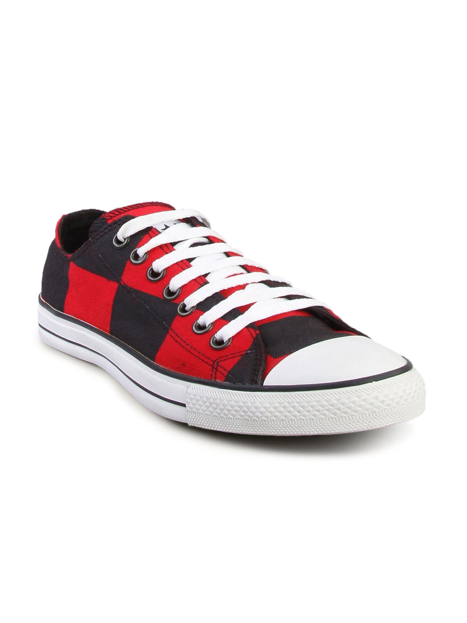
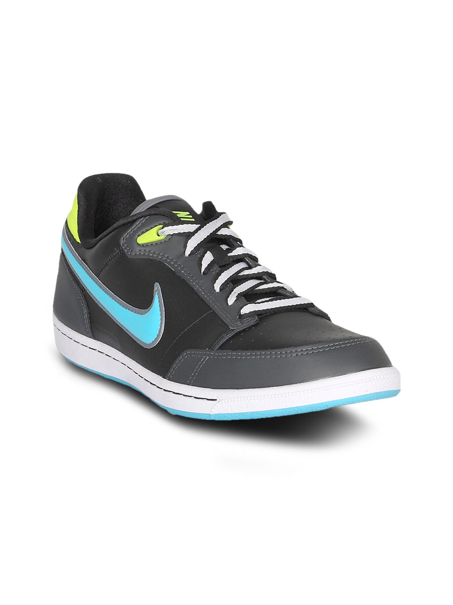
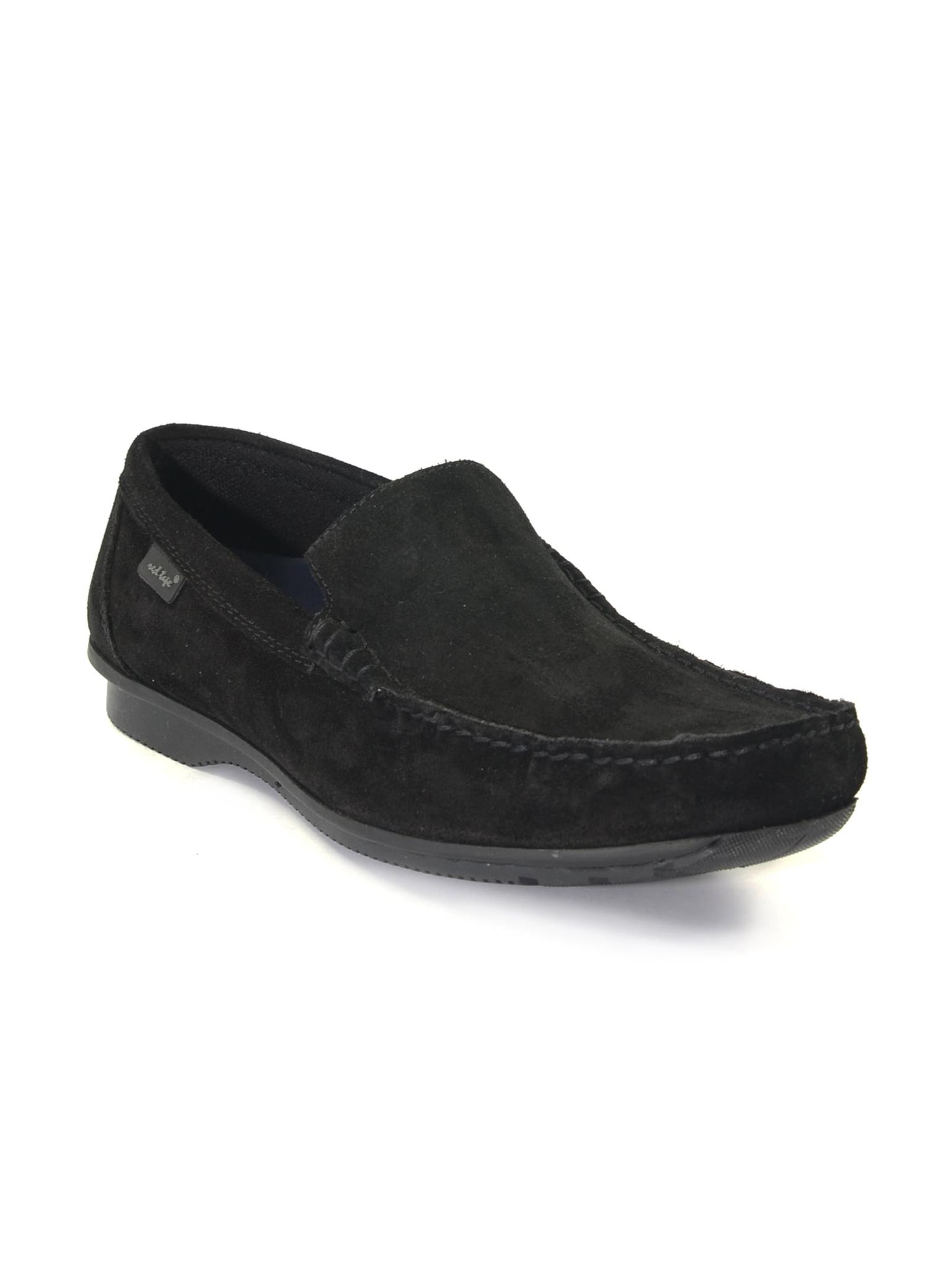
The cell output will display all the pulled shoes from the vector database, showing mostly men's shoes:

http://localhost:3000/notebooks/jupyter_notebook.ipynb

Nike women's transform iii in black pink shoe

Fila men's agony black red shoe

Fila men's passion black red canvas shoe

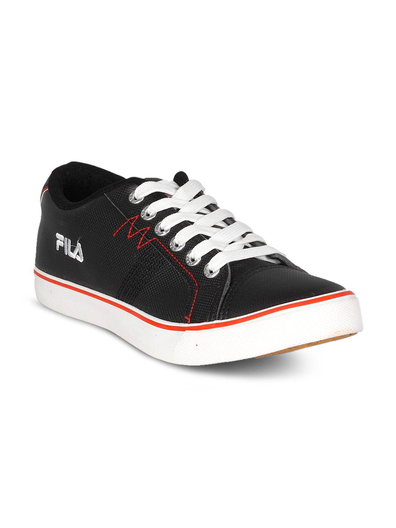
Red tape black men's semi casual shoe

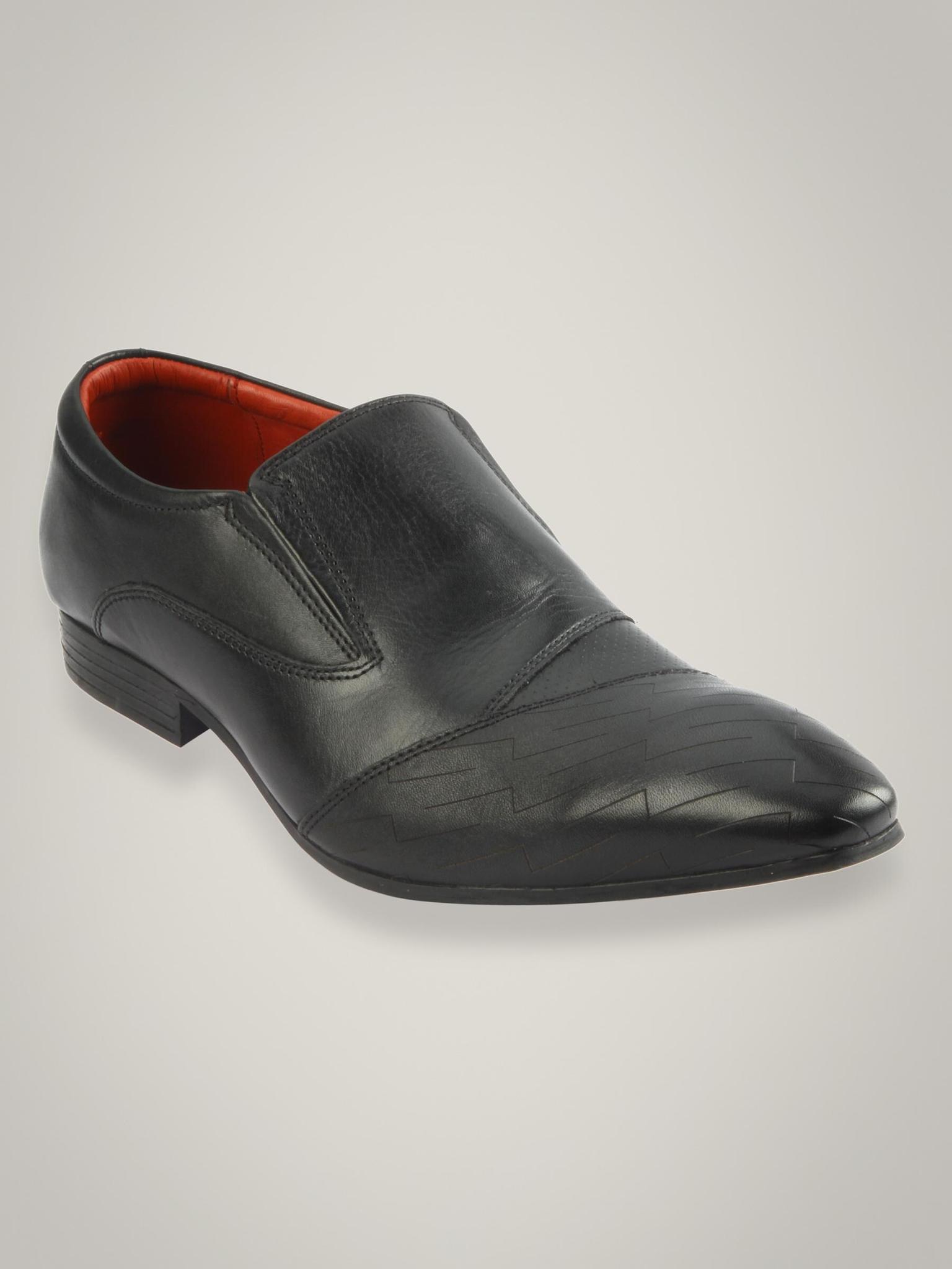
Converse men's chuck taylor big check red black canvas shoe

Red tape men's black formal shoe

Nike women's double team lite black shoe

Red tape men's black casual shoe

Examine query engine results

Looking at the results, the chatbot correctly understands the context of "women's black shoes with red details" and recommends one pair of black shoes with red details.

However, while the LLM correctly identifies that black shoes are requested, it fails to pull multiple black shoes with red details, due to the vector query.

Looking at the pulled shoes, 8 out of 10 are men's shoes, so even though the LLM correctly pulled one relevant shoe, the majority were irrelevant:

The LLM correctly identifies that black shoes are requested but it fails to pull multiple black shoes with red details

Why did the naive chatbot fail?

The naive chatbot struggled with this query because it is designed to vectorize the entire user query and match it against the shoes in the vector database.

While this approach works well for straightforward searches, like the "red shoes" we tried earlier, it has limitations for multiple colors like "black shoes with red details".

Key limitations

Forced query vectorization: By embedding the entire user query, the system treats every word in the query as equally important. This biases the search toward keywords like "women's shoes", "black" or "red", overlooking the multi-color requirement.

In this case, the LLM did notice that the pulled shoes either didn't have red details or were mostly men's shoes but couldn't change the vector query to pull black women's shoes with red details.

Despite that black shoes with red details exist in the dataset, the simple RAG system failed to retrieve them:

Jupyter Notebook
# Verify the dataset for women's black shoes with red details
black_red_shoe_filter = df_shoes[(df_shoes['gender'] == 'women') &
         (df_shoes['color'] == 'black') &
         (df_shoes['color_details'].apply(lambda x: 'red' in x))]
black_red_shoe_filter

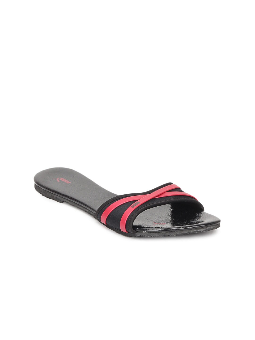
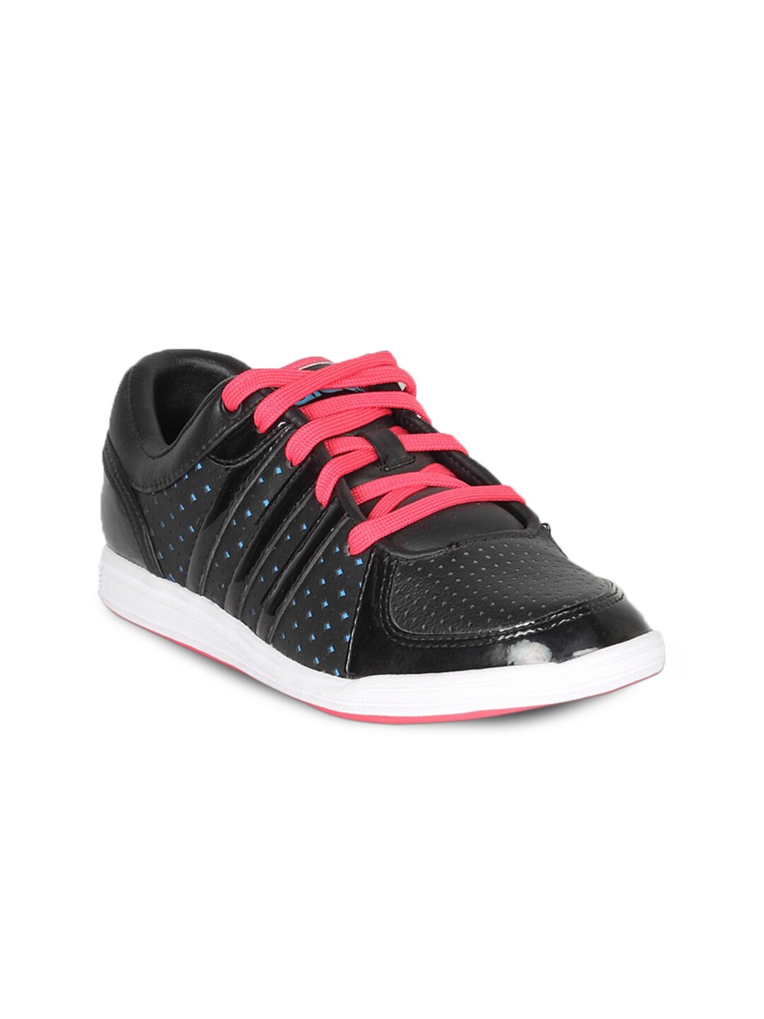
The cell output should show 6 available women's black shoes with red details:

http://localhost:3000/notebooks/jupyter_notebook.ipynb

product_title	gender	product_type	color	usage	color_details	heel_height	heel_type	price_usd	brand	product_id	image
Nike women double team lite black shoes	women	casual shoes	black	casual	['red']	nan	nan	150	nike	706	706.jpg
Puma women saba ballet dc3 black casual shoes	women	casual shoes	black	casual	['red']	nan	nan	170	puma	913	913.jpg
Puma women black crazy slide flats	women	flats	black	casual	['red']	nan	nan	130	puma	959	959.jpg
Catwalk women black heels	women	heels	black	casual	['red']	2	stiletto	70	catwalk	997	997.jpg
Adidas women court sequence black shoe	women	casual shoes	black	casual	['red']	nan	nan	65	adidas	1212	1212.jpg
Hm women black sandals	women	flats	black	casual	['red']	nan	nan	125	hm	1286	1286.jpg

Let's also take a look at the images for these 6 shoes:

Jupyter Notebook
width = 100
images_html = ""
for img_file in black_red_shoe_filter['image']:
    img_path = os.path.join(image_data_path, img_file)
    # Add each image as an HTML <img> tag
    images_html += f'<img src="{img_path}" style="width:{width}px; margin-right:10px;">'
# Display all images in a row using HTML
display(HTML(f'<div style="display: flex; align-items: center;">{images_html}</div>'))

You'll see these shoes in the cell output:

http://localhost:3000/notebooks/jupyter_notebook.ipynb

Query engine limitations

This demonstrates another limitation: when the query embedding doesn't align perfectly with the database, relevant products might be missed.

To address this, let's build an AI agent to enhance query handling.

Create vector store info

We'll start by defining metadata about the vector store we created to allow the AI agent to filter results based on the shoe attributes like:

gender
usage
color
color details
heel heights

This metadata will enhance the AI agent's ability to refine queries and pull relevant shoes.

Since we have numerous colors and usage types, let's create a function that helps up cover all the available colors in our shoe directory.

Add this function to your Jupyter Notebook:

Jupyter Notebook
def generate_options_string(column, is_list_column=False):
    # Extract unique values
    if is_list_column:
        # For list columns, flatten and get unique values
        unique_values = set(item for sublist in column.dropna() for item in sublist)
    else:
        # For non-list columns, get unique values
        unique_values = set(column.dropna())

    # Sort values for consistency
    sorted_values = sorted(unique_values)

    # Handle the string formatting
    if not sorted_values:
        return "No values available"
    elif len(sorted_values) == 1:
        return f"'{sorted_values[0]}'"
    else:
        formatted_values = ", ".join(f"'{value}'" for value in sorted_values[:-1])
        formatted_string = f"Either {formatted_values} or '{sorted_values[-1]}'"
        print(formatted_string)
        return formatted_string

Then, let's run this function for gender, usage and color strings:

Jupyter Notebook
color_string = generate_options_string(df_shoes['color'])
color_details_string = generate_options_string(df_shoes['color_details'], is_list_column=True)
gender_string = generate_options_string(df_shoes['gender'])
usage_string = generate_options_string(df_shoes['usage'])

Running this cell will show an output of each string:

http://localhost:3000/notebooks/jupyter_notebook.ipynb

Jupyter Notebook cell output
'beige', 'black', 'blue', 'bronze', 'brown', 'charcoal', 'copper', 'coral', 'cream', 'gold', 'green', 'grey', 'khaki', 'lavender', 'maroon', 'metallic', 'multi', 'mushroom brown', 'mustard', 'navy blue', 'nude', 'off white', 'olive', 'orange', 'peach', 'pink', 'purple', 'red', 'silver', 'tan', 'taupe', 'teal', 'turquoise blue', 'white' or 'yellow'

'beige', 'black', 'blue', 'bronze', 'brown', 'cream', 'gold', 'green', 'grey', 'maroon', 'metallic', 'multi', 'navy blue', 'off white', 'olive', 'orange', 'pink', 'purple', 'red', 'silver', 'tan', 'teal', 'white' or 'yellow'

'men' or 'women'

'boots', 'casual', 'formal', 'semi formal', 'smart casual' or 'sports'

We're ready to add these strings to our vector store info:

Jupyter Notebook
# Create vector store information
vector_store_info = VectorStoreInfo(
    content_info="shoes in the shoe store",
    metadata_info=[
        MetadataInfo(
            name="gender",
            type="str",
            description=f"Either {gender_string}",
        ),
        MetadataInfo(
            name="usage",
            type="str",
            description=f"Either {usage_string}",
        ),
        MetadataInfo(
            name="color",
            type="str",
            description=f"Either {color_string}",
        ),
        MetadataInfo(
            name="color_details",
            type="List[str]",
            description=f"A list of colors that are in a specified array, filter operator 'in', value has to be List[str] each color being one of: {color_details_string}",
        ),
        MetadataInfo(
            name="price",
            type="int",
            description="The price of the shoes in USD. Must be greater than or equal to 0.",
        ),
    ],
)

Create AI agent tools

Tools are essential for enabling the AI agent to interact with the vector store.

We'll define two tools:

create_metadata_filter: Generates metadata filters for refining the search query
search_footwear_database: Searches the vector database using the query and optional filters

Define metadata filter tool

Let's create the first tool with the ability to create a metadata filters. This tool will have access to the vector store info we just created.

This tool uses

Go ahead and add this tool to your Jupyter Notebook:

Jupyter Notebook
# Define a tool to create metadata filters
def create_metadata_filter(filter_string):
    """
    Creates metadata filter JSON for vector database queries.

    Args:
        filter_string (str): Query string for generating metadata filters.

    Returns:
        str: JSON string of filters.
    """
    class CustomRetriever(VectorIndexAutoRetriever):
        def __init__(self, vector_index, vector_store_info, **kwargs):
            super().__init__(vector_index, vector_store_info, **kwargs)

        def _retrieve(self, query, **kwargs):
            query_bundle = QueryBundle(query_str=query)
            retrieval_spec = self.generate_retrieval_spec(query_bundle)
            return retrieval_spec

    # Separate LLM for generating a filter
    llm_filter = OpenAI_Llama(
        temperature=1, # higher temperature than 0 for creativity
        model="gpt-4o",
        api_key=os.environ["OPENAI_API_KEY"],
        system_prompt="You are a helpful assistant, help the user purchase shoes.",
    )

    custom_retriever = CustomRetriever(
        vector_index=vector_index,
        vector_store_info=vector_store_info,
        llm=llm_filter
    )

    retrieval_spec = custom_retriever._retrieve(filter_string)

    filters_dicts = [{'key': f.key, 'value': f.value, 'operator': f.operator.value} for f in retrieval_spec.filters]
    return json.dumps(filters_dicts)

Define footwear vector database search tool

Next, let's define a tool tht allows our AI agent to search our vector database. Add the following tool to your Jupyter Notebook:

Jupyter Notebook
# Define a tool to search the footwear vector database
def search_footwear_database(query_str, filters_json=None):
    """
    Searches the footwear vector database using a query string and optional filters.

    Args:
        query_str (str): Query string describing the footwear.
        filters_json (Optional[List]): JSON list of metadata filters.

    Returns:
        list: Search results from the vector database.
    """

    # Generate the embedding for the query string
    query_embedding = embed_model._get_query_embedding(query_str)

    # Deserialize from JSON
    if filters_json is None:
        metadata_filters = None
    else:
        metadata_filters = MetadataFilters.from_dicts(filters_json, condition=FilterCondition.AND)


    vector_store_query = VectorStoreQuery(
        query_str=query_str,
        query_embedding=query_embedding,
        alpha=0.5,
        mode='hybrid',
        filters=metadata_filters,
        similarity_top_k=10
    )

    # Execute the query against the vector store
    query_result = vector_store.query(vector_store_query)

    # Create output without embeddings
    nodes_with_scores = []
    for index, node in enumerate(query_result.nodes):
        score: Optional[float] = None
        if query_result.similarities is not None:
            score = query_result.similarities[index]
        nodes_with_scores.append({
            'color': node.metadata['color'],
            'text': node.metadata['text'],
            'gender': node.metadata['gender'],
            'product_type': node.metadata['product_type'],
            'product_id': node.metadata['product_id'],
            'usage': node.metadata['usage'],
            'price': node.metadata['price'],
            'brand': node.metadata['brand'],
            'heel_height': node.metadata.get('heel_height'),  # Add heel_height if present
            'heel_type': node.metadata.get('heel_type'),  # Add heel_type if present
            'similarity_score': score
        })

    return nodes_with_scores

Define agent tools

Now that we have two functions we can use AI agent tools, let's define them as LlamaIndex FunctionTools:

Jupyter Notebook
create_metadata_filters_tool = FunctionTool.from_defaults(
    name="create_metadata_filter",
    fn=create_metadata_filter
)

query_vector_database_tool = FunctionTool.from_defaults(
    name="search_footwear_database",
    fn=search_footwear_database
)

Create AI agent

We'll now define an AI agent capable of reasoning over the data, generating filters and performing refined searches to address customer queries for effectively.

Create AI agent worker

Start by defining the AI agent worker:

Jupyter Notebook
# Create the agent worker
agent_worker = FunctionCallingAgentWorker.from_tools(
    [
        create_metadata_filters_tool,
        query_vector_database_tool,
    ],
    llm=llm,
    verbose=True,
    system_prompt="""\
You are an agent designed to answer customers looking for shoes.\
Please always use the tools provided to answer a question. Do not rely on prior knowledge.\
Drive sales and always feel free to ask a user for more information.\

- Always consider if filters are needed based on the user's query.
- Use the tools provided to answer questions; do not rely on prior knowledge.
- Always feel free to ask a user for more information.

**Example 1:**

User Query: "Hi! I'm going to a party and I'm looking for red women's shoes. Thank you!"

Agent Actions:

1. Determine what query string to use for filters e.g. "red woman's shoes"
2. Call:
   filters_dicts = create_metadata_filter_string("red woman's shoes")
3. Call:
   results = search_footwear_database(query_str='shoes', filters_json=filters_dicts)

**Example 2:**

User Query: "Hi! I'm going to a meeting and I'm looking for formal women's shoes. Thank you!"

Agent Actions:

1. Determine what query string to use for filters e.g. "formal woman's shoes"
2. Call:
   filters_dicts = create_metadata_filter_string("formal woman's shoes")
3. Call:
   results = search_footwear_database(query_str='shoes', filters_json=filters_dicts)

**Example 3:**

User Query: "I'm looking for shoes"

Agent Actions:

1. Ask for more information

**Example 4:**

User Query: "I'm looking for stable heels"

Agent Actions:

1. Determine what query string to use for filters e.g. "women's heels"
2. Call:
   filters_dicts = create_metadata_filter_string("women's heels")
3. Call:
   results = search_footwear_database(query_str='wedges', filters_json=filters_dicts)

Remember to follow these instructions carefully.
""",
)

Create AI agent runner

Next, define the LlamaIndex AI agent AgentRunner:

Jupyter Notebook
agent = AgentRunner(agent_worker)

Test AI agent

Let's test the AI agent by asking for "women's black shoes with red details":

Jupyter Notebook
# Test the agent
agent_response = agent.chat("I need women's black shoes with red details")

You'll progressively see reasoning outputs from the agent when you run the previous cell.

First, you'll see that the agent saves the user message to the memory:

http://localhost:3000/notebooks/jupyter_notebook.ipynb

Jupyter Notebook AI agent cell output

Added user message to memory: I need women's black shoes with red details

Then, you'll see how the AI agent calls the create_metadata_filter tool with the filter string women's black shoes with red details.

http://localhost:3000/notebooks/jupyter_notebook.ipynb

Jupyter Notebook AI agent cell output

=== Calling Function ===
Calling function: create_metadata_filter with args: {"filter_string": "women's black shoes with red details"

Next you'll see the output from the create_metadata_filter tool:

http://localhost:3000/notebooks/jupyter_notebook.ipynb

Jupyter Notebook AI agent cell output

=== Function Output ===
[{"key": "gender", "value": "women", "operator": "=="}, {"key": "color", "value": "black", "operator": "=="}, {"key": "color_details", "value": ["red"], "operator": "in"}]

After that, the AI agent uses the generated filter as input in the search_footwear_database tool:

http://localhost:3000/notebooks/jupyter_notebook.ipynb

Jupyter Notebook AI agent cell output

=== Calling Function ===
Calling function: search_footwear_database with args: {"query_str": "shoes", "filters_json": [{"key": "gender", "value": "women", "operator": "=="}, {"key": "color", "value": "black", "operator": "=="}, {"key": "color_details", "value": ["red"], "operator": "in"}]}

You'll also see the full vector database response:

http://localhost:3000/notebooks/jupyter_notebook.ipynb

Jupyter Notebook AI agent cell output

=== Function Output ===
[{'color': 'black', 'text': 'Puma women saba ballet dc3 black casual shoes', 'gender': 'women', 'product_type': 'casual shoes', 'product_id': 913, 'usage': 'casual', 'price': 170, 'brand': 'puma', 'heel_height': None, 'heel_type': None, 'similarity_score': 1.69973636}, {'color': 'black', 'text': 'Nike women double team lite black shoes', 'gender': 'women', 'product_type': 'casual shoes', 'product_id': 706, 'usage': 'casual', 'price': 150, 'brand': 'nike', 'heel_height': None, 'heel_type': None, 'similarity_score': 1.69866252}, {'color': 'black', 'text': 'Hm women black sandals', 'gender': 'women', 'product_type': 'flats', 'product_id': 1286, 'usage': 'casual', 'price': 125, 'brand': 'hm', 'heel_height': None, 'heel_type': None, 'similarity_score': 1.22095072}, {'color': 'black', 'text': 'Catwalk women black heels', 'gender': 'women', 'product_type': 'heels', 'product_id': 997, 'usage': 'casual', 'price': 70, 'brand': 'catwalk', 'heel_height': 2.0, 'heel_type': 'stiletto', 'similarity_score': 1.1970259}, {'color': 'black', 'text': 'Adidas women court sequence black shoe', 'gender': 'women', 'product_type': 'casual shoes', 'product_id': 1212, 'usage': 'casual', 'price': 65, 'brand': 'adidas', 'heel_height': None, 'heel_type': None, 'similarity_score': 1.18892908}, {'color': 'black', 'text': 'Puma women black crazy slide flats', 'gender': 'women', 'product_type': 'flats', 'product_id': 959, 'usage': 'casual', 'price': 130, 'brand': 'puma', 'heel_height': None, 'heel_type': None, 'similarity_score': 1.16182387}]

Finally you'll see the LLM response after reasoning over the vector database output data:

http://localhost:3000/notebooks/jupyter_notebook.ipynb

Jupyter Notebook AI agent cell output
== LLM Response ===
Here are some women's black shoes with red details that you might like:

1. **Puma Women Saba Ballet DC3 Black Casual Shoes**

 - Price: $170
 - Brand: Puma
 - Type: Casual Shoes

2. **Nike Women Double Team Lite Black Shoes**

 - Price: $150
 - Brand: Nike
 - Type: Casual Shoes

3. **HM Women Black Sandals**

 - Price: $125
 - Brand: HM
 - Type: Flats

4. **Catwalk Women Black Heels**

 - Price: $70
 - Brand: Catwalk
 - Type: Heels
 - Heel Height: 2.0 inches
 - Heel Type: Stiletto

5. **Adidas Women Court Sequence Black Shoe**

 - Price: $65
 - Brand: Adidas
 - Type: Casual Shoes

6. **Puma Women Black Crazy Slide Flats**
 - Price: $130
 - Brand: Puma
 - Type: Flats

Let me know if you need more information on any of these options!

Visualize the AI agent's recommendations

Let's go ahead create a function that visualizes the AI agent's recommended shoes:

Jupyter Notebook
def visualize_agent_response(agent_response, image_folder_path=None, img_width=150, threshold=98):
    """
    Visualizes products from agent response if they match (fuzzily) names in an unstructured string.

    Args:
    - agent_response: Agent response.
    - image_folder: Path to the folder containing product images.
    - img_width: Width of the product images in the visualization.
    - threshold: Minimum similarity score for fuzzy matching.

    Returns:
    - None: Displays the visualization directly in the notebook.
    """
    if image_folder_path is None:
        raise ValueError("You must specify an image folder path.")

    # Extract product names from raw output and make them lowercase
    products = [product['text'].lower() for product in agent_response.sources[1].raw_output]

    # Prepare HTML content for visualization
    html_content = "<div style='display: flex; flex-wrap: wrap; gap: 20px;'>"

    # Loop through the products and match with unstructured string
    for product in agent_response.sources[1].raw_output:
        product_name = product['text'].lower()

        # Perform fuzzy matching
        match = process.extractOne(product_name, [agent_response.response.lower()], scorer=fuzz.partial_ratio)
        if match and match[1] > threshold:  # If a match is found and meets the threshold
            # Generate image path based on product_id
            image_path = os.path.join(image_folder_path, f"{product['product_id']}.jpg")

            # Append product info and image to HTML content
            html_content += f"""
                <div style="text-align: center;">
                    <p>{product['text']}</p>
                    <img src='{image_path}' width='{img_width}px' style="padding: 5px;"/>
                </div>
            """

    # Close the main div
    html_content += "</div>"

    # Display the content as HTML
    display(HTML(html_content))

Then go ahead and call the function:

Jupyter Notebook
# Call the function
visualize_agent_response(agent_response, image_folder_path=image_data_path)

You should see these 6 shoes in the cell output:

http://localhost:3000/notebooks/jupyter_notebook.ipynb

Puma women saba ballet dc3 black casual shoes

Nike women double team lite black shoes

Hm women black sandals

Catwalk women black heels

Adidas women court sequence black shoe

Puma women black crazy slide flats

Compare AI agent recommendations with available shoes

Looking back at when we filtered our shoe directory for black women's shoes with red details, we received 6 pair of shoes:

Jupyter Notebook
# Verify the dataset for women's black shoes with red details
black_red_shoe_filter = df_shoes[(df_shoes['gender'] == 'women') &
         (df_shoes['color'] == 'black') &
         (df_shoes['color_details'].apply(lambda x: 'red' in x))]

width = 100
images_html = ""
for img_file in black_red_shoe_filter['image']:
    img_path = os.path.join(image_data_path, img_file)
    # Add each image as an HTML <img> tag
    images_html += f'<img src="{img_path}" style="width:{width}px; margin-right:10px;">'
# Display all images in a row using HTML
display(HTML(f'<div style="display: flex; align-items: center;">{images_html}</div>'))

http://localhost:3000/notebooks/jupyter_notebook.ipynb

The AI agent reply includes all of these 6 pair of shoes:

=== LLM Response ===
Here are some women's black shoes with red details that you might like:

1. **Puma Women Saba Ballet DC3 Black Casual Shoes**

 - Price: $170
 - Brand: Puma
 - Type: Casual Shoes

2. **Nike Women Double Team Lite Black Shoes**

 - Price: $150
 - Brand: Nike
 - Type: Casual Shoes

3. **HM Women Black Sandals**

 - Price: $125
 - Brand: HM
 - Type: Flats

4. **Catwalk Women Black Heels**

 - Price: $70
 - Brand: Catwalk
 - Type: Heels
 - Heel Height: 2.0 inches
 - Heel Type: Stiletto

5. **Adidas Women Court Sequence Black Shoe**

 - Price: $65
 - Brand: Adidas
 - Type: Casual Shoes

6. **Puma Women Black Crazy Slide Flats**
 - Price: $130
 - Brand: Puma
 - Type: Flats

Let me know if you need more information on any of these options!

AI agent response visualized:

http://localhost:3000/notebooks/jupyter_notebook.ipynb

Detailed AI agent workflow

AI agent workflow

When we ask the AI agent for women's black shoes with red details, the agent takes the following steps:

1. Tool invocation

Calls the create_metadata_filter tool with the argument women's black shoes with red details, which generates the following metadata filter:

[
    {"key": "gender", "value": "women", "operator": "=="},
    {"key": "color", "value": "black", "operator": "=="},
    {"key": "color_details", "value": ["red"], "operator": "in"}
]

Calls the search_footwear_database tools with the query string shoes and the generated filter.

This refines the search to only include black women's shoes with red details.

2. Response generation

The AI agent looks through the retrieved vector database results and provide a response with recommended shoes:

Here are some women's black shoes with red details that you might like:

1. **Puma Women Saba Ballet DC3 Black Casual Shoes**
   - Price: $170
   - Brand: Puma
   - Type: Casual Shoes

2. **Nike Women Double Team Lite Black Shoes**
   - Price: $150
   - Brand: Nike
   - Type: Casual Shoes

3. **HM Women Black Sandals**
   - Price: $125
   - Brand: HM
   - Type: Flats

4. **Catwalk Women Black Heels**
   - Price: $70
   - Brand: Catwalk
   - Type: Heels
   - Heel Height: 2.0 inches
   - Heel Type: Stiletto

5. **Adidas Women Court Sequence Black Shoe**
   - Price: $65
   - Brand: Adidas
   - Type: Casual Shoes

6. **Puma Women Black Crazy Slide Flats**
   - Price: $130
   - Brand: Puma
   - Type: Flats

Let me know if you need more information on any of these options!

The AI agent looks through the retrieved vector database results and provide a response with recommended shoes

How Did the AI Agent Succeed?

Understands multiple color request
Applies filters to return all matches, not just the first found
Leverages metadata (color_details) to ensure accurate results

Key Takeaways

Naive Chatbot Limitation

Finds limited or no results due to lack of multiple color filtering

AI Agent Advantages

Accurately applies multiple color filters
Shows all products that fit the user's request
Enhances the shopping experience with full, accurate results

Conclusion

When users specify multiple color requirements like black shoes with red details, naive chatbots fail to apply proper filters and return only partial matches.

AI agents, on the other hand, use metadata filtering and reasoning to find all suitable options, improving both accuracy and user satisfaction.

Introduction​

Prerequisites​

Introducing SoleMates​

Challenge: handling multi-color queries​

Scenario​

Install dependencies​

Load shoe data​

Cost of vectorization​

Pre-embedded dataset​

Prepare Amazon Bedrock for embedding generation​

Why use AWS Titan?​

Getting started with Amazon Bedrock​

Set up AWS Bedrock client​

Generate embeddings​

Create a dictionary with product data​

Create LlamaIndex Documents​

Initialize Pinecone​

List current indexes​

Create new index​

Inspect Pinecone​

Initialize Pinecone index​

Create Pinecone vector store​

Create an ingestion pipeline​

Run the ingestion pipeline​

Inspect your Pinecone index​

Test querying the vector store​

Query the vector database directly​

Why use a simple retriever?​

Create a function to request AWS Titan embeddings​

Create custom embedding class​

Instantiate the custom class​

Create a simple retriever​

Create retriever​

Why query the vector database directly with a simple retriever?​

Why this step matters​

Query the vector store​

Function to visualize the vector database pull​

Visualize shoes​

Examine the shoes​

Why not keep using the index alone?​

Test the naive query​

Limitations of a naive RAG system​

Overcome naive RAG limitations: create a vector index query engine​

Initialize LLM​

Create query engine​

Test query engine with today's challenge: black shoes with red details​

Examine query engine results​

Why did the naive chatbot fail?​

Key limitations​

Query engine limitations​

Create vector store info​

Create AI agent tools​

Define metadata filter tool​

Define footwear vector database search tool​

Define agent tools​

Create AI agent​

Create AI agent worker​

Create AI agent runner​

Test AI agent​

Visualize the AI agent's recommendations​

Compare AI agent recommendations with available shoes​

Detailed AI agent workflow​

AI agent workflow​

How Did the AI Agent Succeed?​

Key Takeaways​

Naive Chatbot Limitation​

AI Agent Advantages​

Conclusion​

Introduction

Prerequisites

Introducing SoleMates

Challenge: handling multi-color queries

Scenario

Install dependencies

Load shoe data

Cost of vectorization

Pre-embedded dataset

Prepare Amazon Bedrock for embedding generation

Why use AWS Titan?

Getting started with Amazon Bedrock

Set up AWS Bedrock client

Generate embeddings

Create a dictionary with product data

Create LlamaIndex Documents

Initialize Pinecone

List current indexes

Create new index

Inspect Pinecone

Initialize Pinecone index

Create Pinecone vector store

Create an ingestion pipeline

Run the ingestion pipeline

Inspect your Pinecone index

Test querying the vector store

Query the vector database directly

Why use a simple retriever?

Create a function to request AWS Titan embeddings

Create custom embedding class

Instantiate the custom class

Create a simple retriever

Create retriever

Why query the vector database directly with a simple retriever?

Why this step matters

Query the vector store

Function to visualize the vector database pull

Visualize shoes

Examine the shoes

Why not keep using the index alone?

Test the naive query

Limitations of a naive RAG system

Overcome naive RAG limitations: create a vector index query engine

Initialize LLM

Create query engine

Test query engine with today's challenge: black shoes with red details

Examine query engine results

Why did the naive chatbot fail?

Key limitations

Query engine limitations

Create vector store info

Create AI agent tools

Define metadata filter tool

Define footwear vector database search tool

Define agent tools

Create AI agent

Create AI agent worker

Create AI agent runner

Test AI agent

Visualize the AI agent's recommendations

Compare AI agent recommendations with available shoes

Detailed AI agent workflow

AI agent workflow

How Did the AI Agent Succeed?

Key Takeaways

Naive Chatbot Limitation

AI Agent Advantages

Conclusion